Product Assurance Run-time – Product Quality Supervision

General Description
Product Assurance Runtime objective is to perform actions to ensure the quality and suitability of a product, based on the data obtained in the manufacturing process, or in the inspection of the products once they are finished. Internally, the Product Assurance Runtime is divided in two different tasks:
Product Quality Prediction, which predicts the quality of the product and anticipate possible defects arising during manufacturing process: this can have a double advantage, on one hand avoiding unnecessary further manufacturing steps, on the other it can help to redefine production parameters or initial conditions (materials) as corrective actions to restore quality threshold
Supervision, which monitors each individual part along the entire supply chain, collecting all relevant information in the process, with the aim of identifying critical trends that might result in possible downstream defects
Both tasks are based on Artificial Intelligence (AI) and Big Data techniques. However, the approaches vary as the desired results are different, and the techniques, or the way they are applied, are also different.
The following sections focus on the description of specific features, requirements, and use of Supervision task.
The following table shows the assets available:
| Resource | Location |
|---|---|
| Source Code | Link |
| Latest Release (Model Deployment Manager) | v1.0.3 |
| Open API Spec (Data Processor) | Link |
| Video | |
| Further Guidance |
|
| Related Datasets |
|
| Additional Links |
|
| Generation date of this content | 14 May 2021 |
Screenshots
The following images are illustrative screen shots of the component.

Figure 1. Model Deployment Manager
Component Author(s)
| Company Name | ZDMP Acronym | Website | Logo |
|---|---|---|---|
| Instituto Tecnológico de Informática | ITI | https://www.iti.es/ |  |
| Ceteck Tecnológica S.L. | CET | http://www.grupoceteck.com |  |
Commercial Information
| Resource | Location |
|---|---|
| IPR Link | |
| Price | [For determination at end of project] |
| Licence | [For determination at end of project] |
| Privacy Policy | [For determination at end of project] |
| Volume license | [For determination at end of project] |
Architecture Diagram
The following diagram shows the position of this component in the ZDMP architecture.
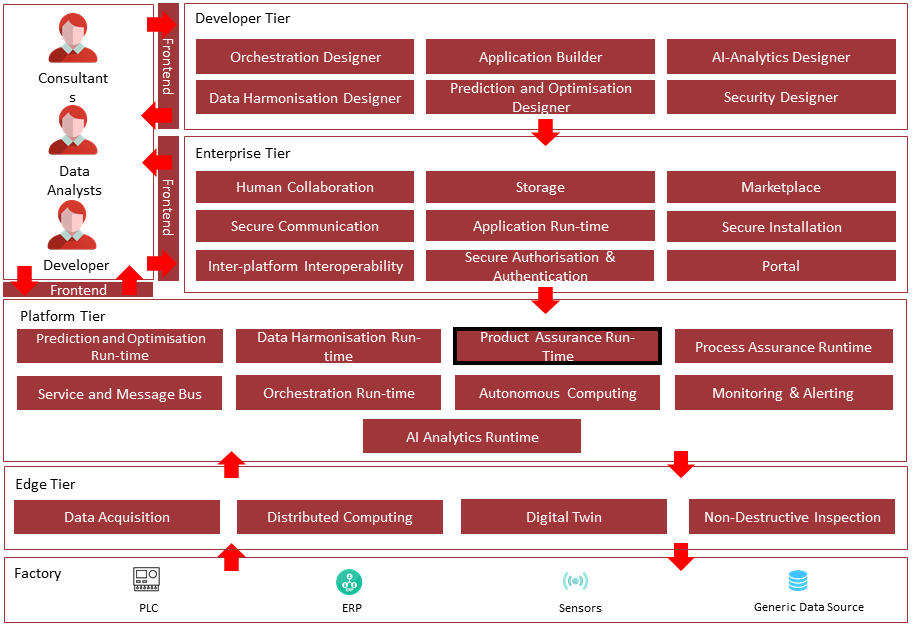
Figure 2. Position of Component in ZDMP Architecture
Benefits
General
The Supervision component has several benefits for the Data Analysts, but also for generic programmers with low knowledge about Machine Learning. It provides an abstraction layer that allows them to use well known algorithms and deploy them directly to the AI Analytics Runtime, using the Model Deployment Manager. These are the main benefits of using the Supervision component:
Access to predefined algorithms to solve common problems in the industry
Ability to customize those algorithms to fit in specific problems
Abstraction layer for the software engineering tasks, thanks to the integration with the AI Analytics Runtime. This includes:
Docker image construction
API wrapping
Data source connections (Message Bus, Storage, etc)
Security monitoring
Model Deployment Manager
Defines the manifesto, which contains all the needed information to define every aspect of the model, allowing the models to be deployed through the AI Analytics Run-time
Friendly user interface, allowing the user to easily generate the manifesto
Within the Model Deployment Manager interface is integrated the user interface of the Data Processor
The user selects the inputs and outputs needed to execute the model to upload, and at the same time configures the Data Processor transformations for the selected inputs or outputs
Data Processor
Composed by a set of intrinsic meaningful transformations
Support streaming transformations and batch transformations (configurable)
Integrates with AI Analytics Run-time and takes profit of AI Analytics integrations:
Secure Authentication and Authorization
Message Bus
Infrastructure management
Manifest definition
Reducing the coupling between components allows Data Processor to focus their efforts to add more complex data transformations
Features
Supervision Description
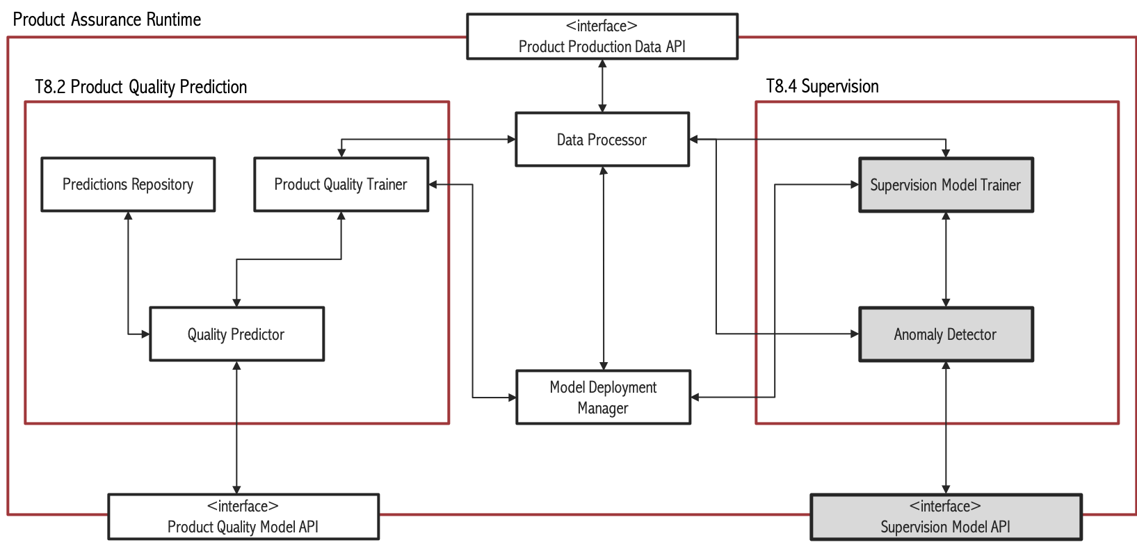
Figure 3. Subsystem architecture of Supervision task
The main objective of the Supervision task is to provide real time predictions regarding the result of a manufacturing process, and whether there are anomalies present or not by using Artificial Intelligence and Big Data techniques. Here one can differentiate two scenarios: Unsupervised and supervised. In the unsupervised scenario, no product quality variable is available. This can be somewhat common in SMEs because of lack of resources to perform quality tests. Another cause could be technical difficulties to obtain product quality data. In the supervised scenario there are one or more variables that measure product quality. In those cases, it is possible to relate process conditions to those quality measures using Machine Learning algorithms. The supervised scenario can be split into two cases: classification (when the quality measure is binary or categorical) and regression (that refers to the case in which the quality variable is quantitative).
On the other hand, ZDMP must be able to cope with a scenario in which large volumes of streaming data and product changes are present. In this scenario, classical batch machine learning algorithms are not the best approach. Batch learning tries to process all data simultaneously and does not integrate new data into already existing models, trying to rebuild new models from scratch. This approach is very time consuming and leads to obsolete models and large volumes of unprocessed data. On the contrary, incremental learning fits to this scenario since it continuously integrates new data into existing models, being less time and space consuming than batch learning.
Another issue to consider is the imbalanced problem. One of the objectives of ZDMP is to detect abnormal situations that could derive into faulty products. Good products are more frequent than bad ones, which, in terms of machine learning, provokes an imbalanced dataset, that is, a dataset in which the majority class is 100 or 1000 times greater than the minority class. This can result in inferior performance of the classical machine learning models because the majority class may dominate the learning process producing biased results. Some of the algorithms implemented include strategies especially designed to deal with this problem.
Every process in an industry environment has its own peculiarities. For this reason, this component provides different technologies, such as PCA, Incremental Online Learning, etc to give versatility to the final users. In addition, the data produced by every manufacturing process will vary and, depending on that, component may use a tool or another, which allows versatility.
The features to achieve the functionality of this component are itemised below and explained thereafter.
Model Deployment Manager
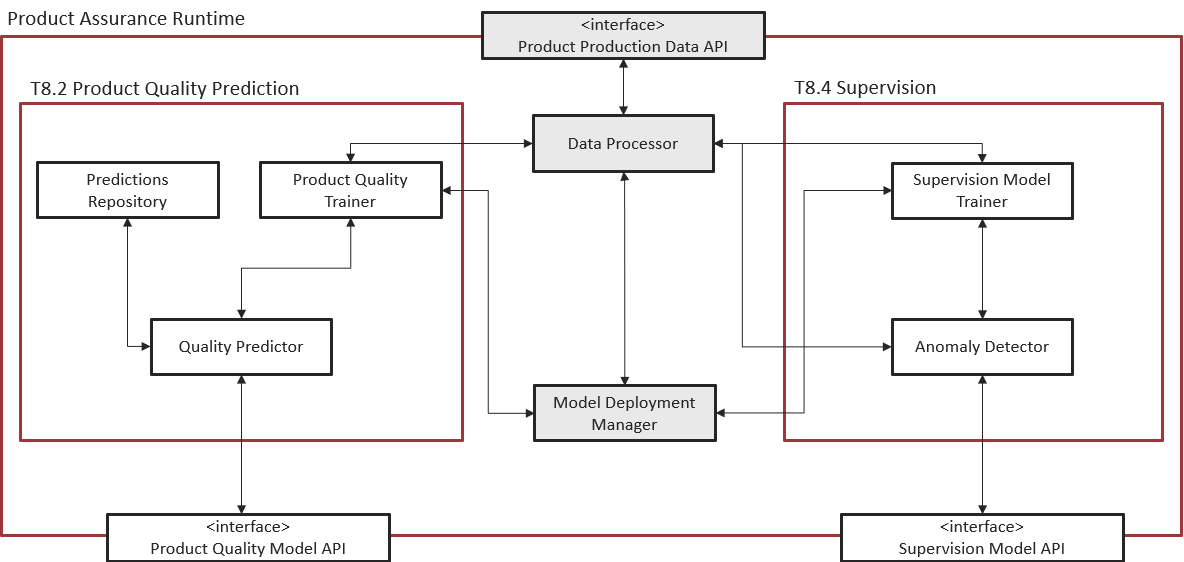
Figure 4. Subsystem architecture of Model Deployment Manager and Data Processor
Provides the user interface to ease the generation of the manifesto. The manifesto contains all the needed information to execute the model
Integrates with AI Analytics Run-time to allow the user to upload models with the expected structure within AI Analytics Run-time, and to run/stop models
Integrates with Data Processor to allow the user configure data transformations
Integrates with Product Assurance Run-time - Product Quality Prediction task and also Supervision task, to show/select the models available (which are explained in Unsupervised Anomaly Detection, Classification and Regression sections)
Integrates with Secure Authentication and Authorization to allow the security configuration of the model
Data Processor
Define a rules system to transform incoming data
Allows the temporally alignment of data
The transformations configured by the user through the Model Deployment Manager user interface are collected in the manifesto; the Model Deployment Manager sends the manifesto to the AI Analytics Run-time and with this information the AI Analytics Run-time calls the Data Processor API to perform the selected transformations
These are the data transformations implemented at this stage:
Scale by factor: Values are multiplied by a factor introduced by the user. It is used in conversion of units of measure and scaling data to fit into the adequate range
Change time zone: Data from different time zones need to be aligned. The solution is to change every timestamp from the origin time zone to a common time zone
Change sample frequency: Data collected with different sample frequency need to have the same frequency
System Requirements
Model Deployment Manager
The component may be run on any platform that supports Docker images.
Data Processor
The component may be run on any platform that supports Docker images.
Associated ZDMP services
Required
The following ZDMP components are required for the correct execution of this component:
Optional
These are the optional ZDMP components:
Installation
Model Deployment Manager
Download the zip file from this link: Download
Create a folder named “Model Deployment Manager” and extract there the content of the zip file downloaded. The folder structure should be:
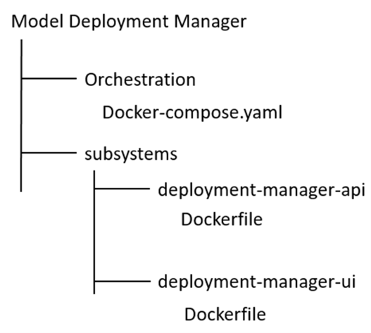
Run Docker Desktop
Run PowerShell, navigate through folders until folder “orchestration” and then write the command: Docker-compose up. Now the Model Deployment Manager is running
Download Secure Authentication and Authorization software from this link: Download. In the same way as in the previous steps, extract the files, run PowerShell, navigate through folders until folder “orchestration” and execute the command: Docker-compose up. Now the component Secure Authentication and Authorization is running
Install Data Processor as described in the next section
Data Processor
Download the zip file from this link: Download
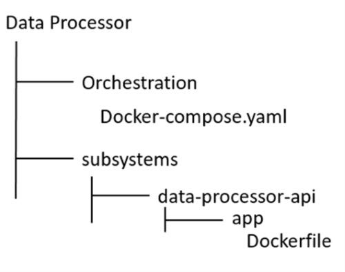
Create a folder named ”Data Processor” and extract there the content of the file downloaded. The folder structure should be:
Run Docker Desktop
Run PowerShell, navigate through folders until folder “orchestration” and then write the command: Docker-compose up
How to use
Model Deployment Manager
The Model Deployment Manager user interface allows the user to upload a model with the expected structure into the AI Analytics Runtime, selecting input and output signals needed to run the model. As anticipated in the Features section, this user interface allows configuring data transformations available in the Data Processor for each of the input and output signals. When the user completes the sequence of steps established in the Model Deployment Manager the result is a zip file that contains the model to be executed in the AI Analytics Run-time and the manifesto which is a JSON file containing the data structure and information needed for the AI Analytics Run-time to execute the model.
Once the installation steps are executed as previously described, the Model Deployment Manager UI is accessible through the browser at http://localhost:5007
Main screen: Your Deployments
This screen shows to the user a list of the available models (those to which the user has permission) within the AI Analytics Runtime. As shown in the image below, the user can see the status of the models (running, stopped, error).
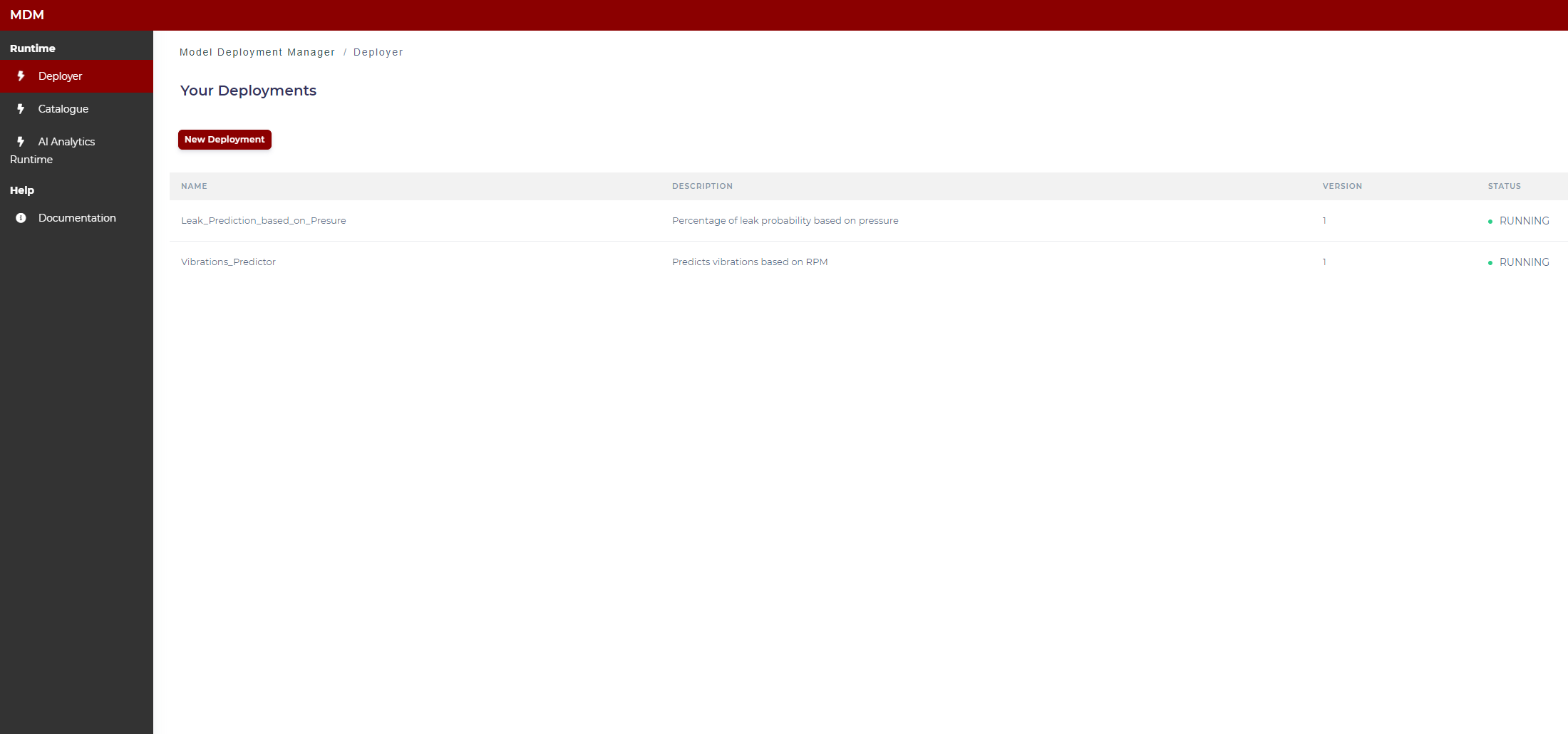
Figure 5. Available models
In the side menu on the left, there are the following items:
- Deployer: It opens the main screen of the Model Deployment Manager as shown in Figure 5
AI Analytics Run-time: It links with the AI Analytics Run-time, opening it in another browser window
Catalogue: It opens the Catalogue which contains the algorithms implemented for the Production Supervision subcomponent. As shown in Figure 6, the algorithms are divided into three main categories: Unsupervised, classification and regression. Unsupervised algorithms refer to the case in which a quality variable is not available. The classification algorithms are applied to the case in which the quality variable is binary (type Yes / No) or categorical (with several classes). Regression algorithms address the problem in which the quality variable is quantitative. The user can download any model from the catalogue (clicking on the corresponding “download” button) and use it as a template for the model that will be finally deployed in the AI Analytics Run-time through the Model Deployment Manager. This is described in the following “Step 2: Upload the model” section
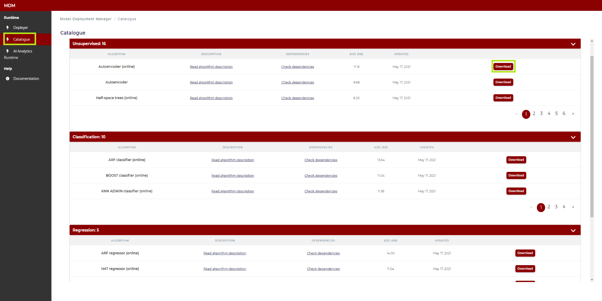
Figure 6. Catalogue
In order to upload a new model, the user clicks on “New Deployment” as shown in the following image:
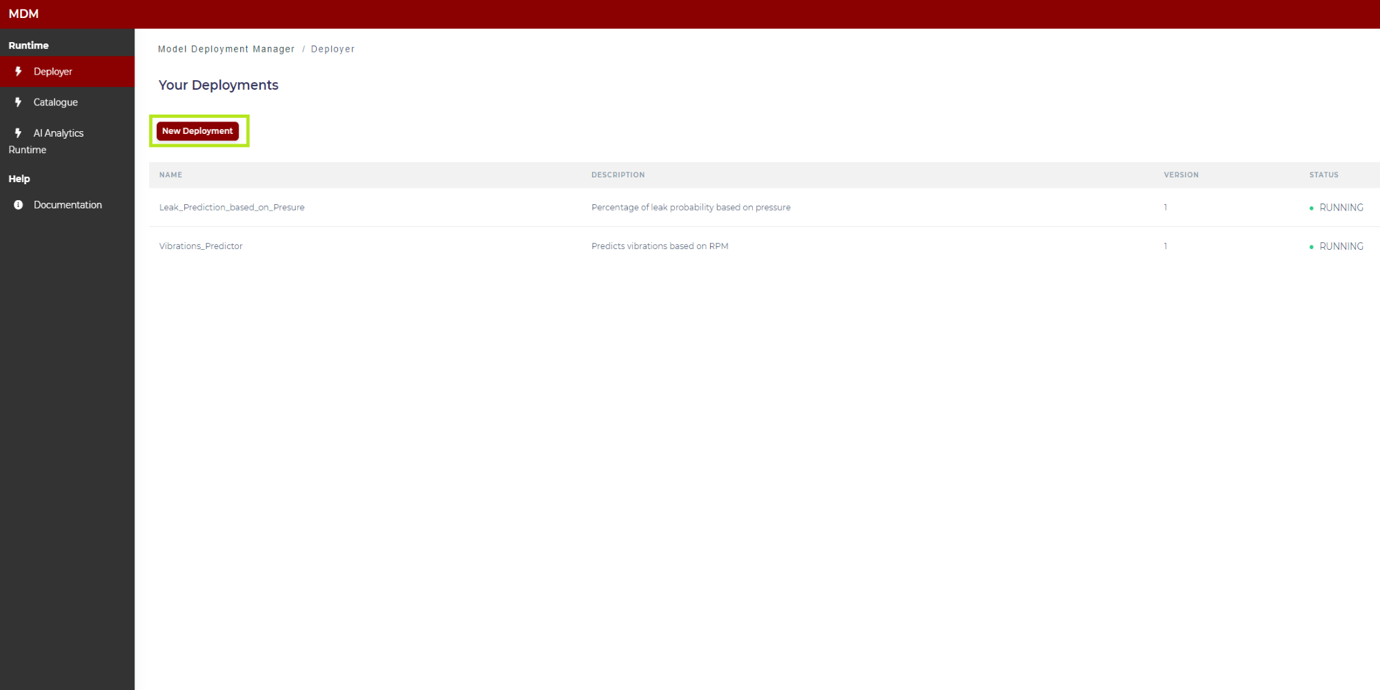
Figure 7. Creation of a new deployment
Then the configuration wizard starts, with the steps described in the following sections.
Step 1: Choose the machine learning type of the model
At this stage of development, the only model type available for the models to be uploaded by the user is python code type, so select it and click on “Next”. Firther types of models foreseen in the platform will be soon available; the first are the ones resulting from the AI Analytics Designer based on H2O framework, while the second ones are the so called “Docker layer” models, built from the Prediction and Optimization Run-time base image, or optionally using the Prediction and Optimization Designer.
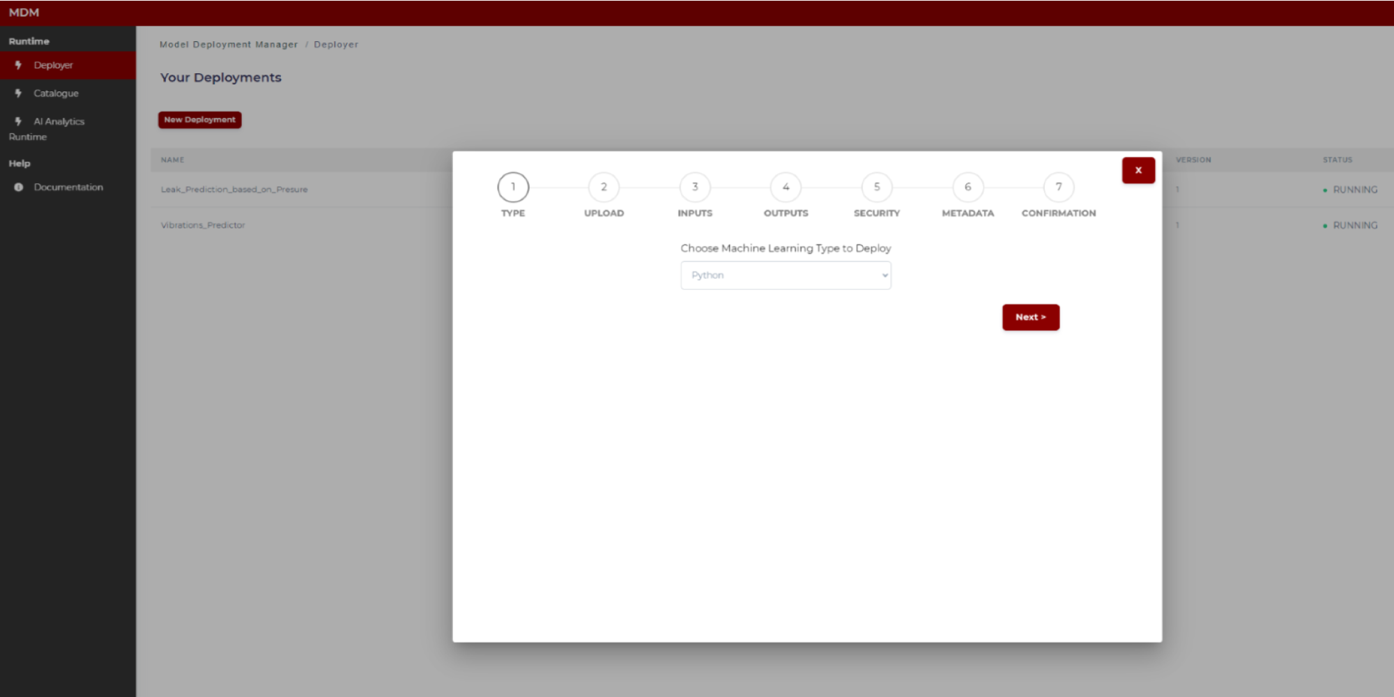
Figure 8. Machine learning model selection
Step 2: Upload the model
In this step the user uploads the desired model code from the local computer and inserts the corresponding parameters if necessary. To explain it better, in the following image the different sections of this screen are marked and numbered in green:
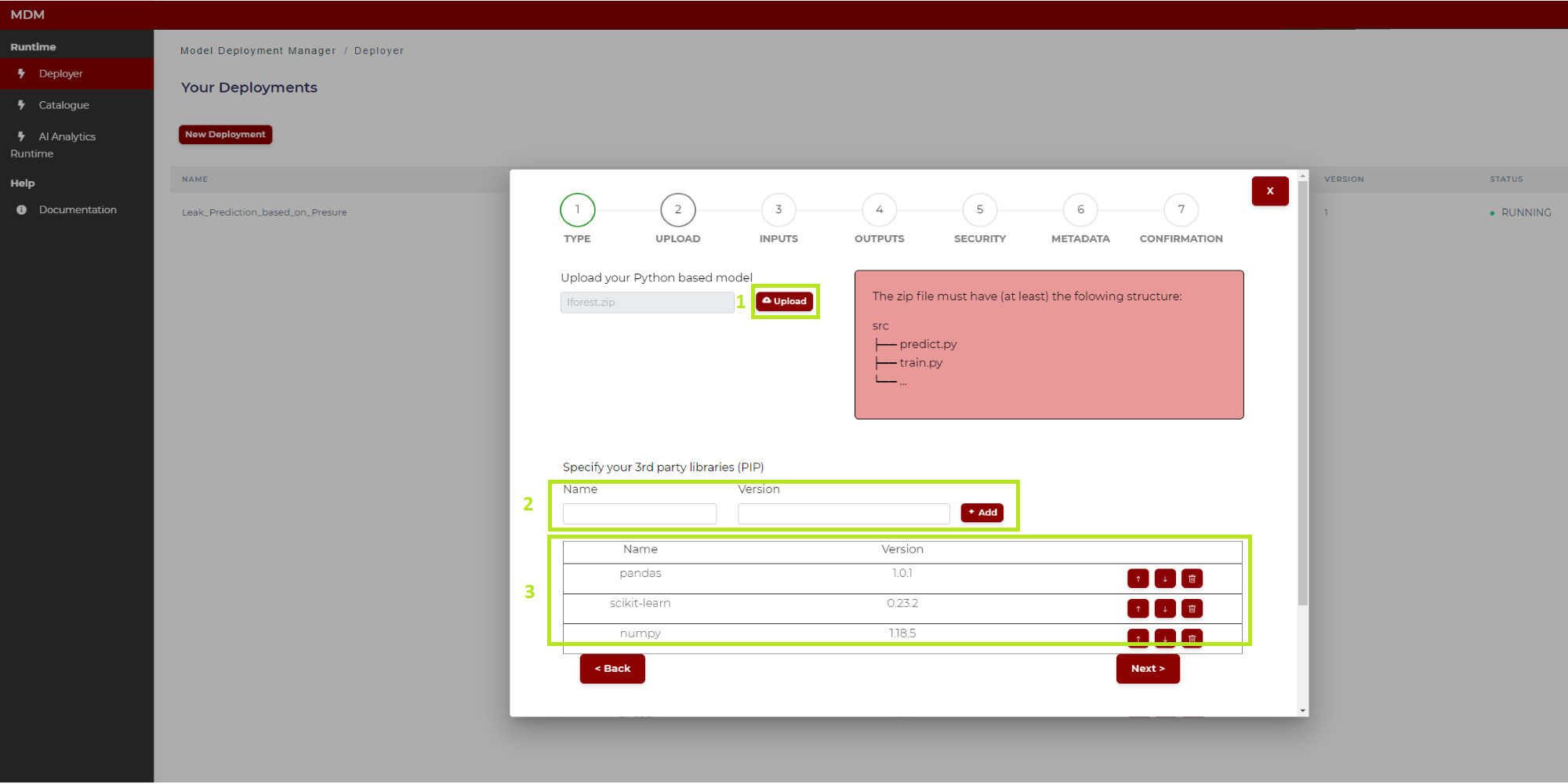
Figure 9. Model uploading
1: Click on “Upload” and select from the local computer the zip file which contains the model to be uploaded, for example one previously downloaded from the Catalogue described above. As shown on the right, the compressed file must have at least a folder named “src” and into this folder the python files “train.py” and “predict.py”, for the two machine learning phases to be run in the AI Analytics Run-time, respectively training and inference. For more information about these two python codes see below the “General Considerations” section and the ones which follow, where parameters and more details for these functions are described for each machine learning algorithm available in the catalogue. If the user has an already trained model, the correspondent .pkl file must be included into the “src” folder, and the “train.py” file is no more needed: note that this is exactly the kind of output which is described in the Export Model section of the Quality Prediction Designer, and which is automatically packaged as a result of the training operation
2: In this field the user types the name and version of the python third party libraries, if needed. After typing the library name and version, click on “Add” and it is added in the list “3”. In case the user puts the corresponding file “requirements.txt” (which contains the python libraries) into the “src” folder, then the user does not need to fill this section, as the libraries contained in the file “requirements.txt will be included automatically in the manifest
3: All the libraries added in “2” are shown in this list. The user can delete a row if needed
Step 3: Inputs
In this step the user configures the input data sources that will feed the model. These are the possible configurations for input data channels for training and/or prediction phases:
Training – Historic Data: Defines the dataset to be used in the training phase
Prediction – REST API: Trained model will be wrapped inside a REST API, so generating an exposed endpoint to be called for prediction
Training/Prediction – Message Bus: Deployed model will listen to the given topics. In the prediction phase published data will be consumed by the predict function to make an inference, while in the training phase data will be used for on-line learning to release and updated version of the trained model
The screen is divided into two parts: Training phase and prediction phase. If the model does not need a training phase, the user clicks on “skip training phase” as shown in the following image, and then the training section disappears:
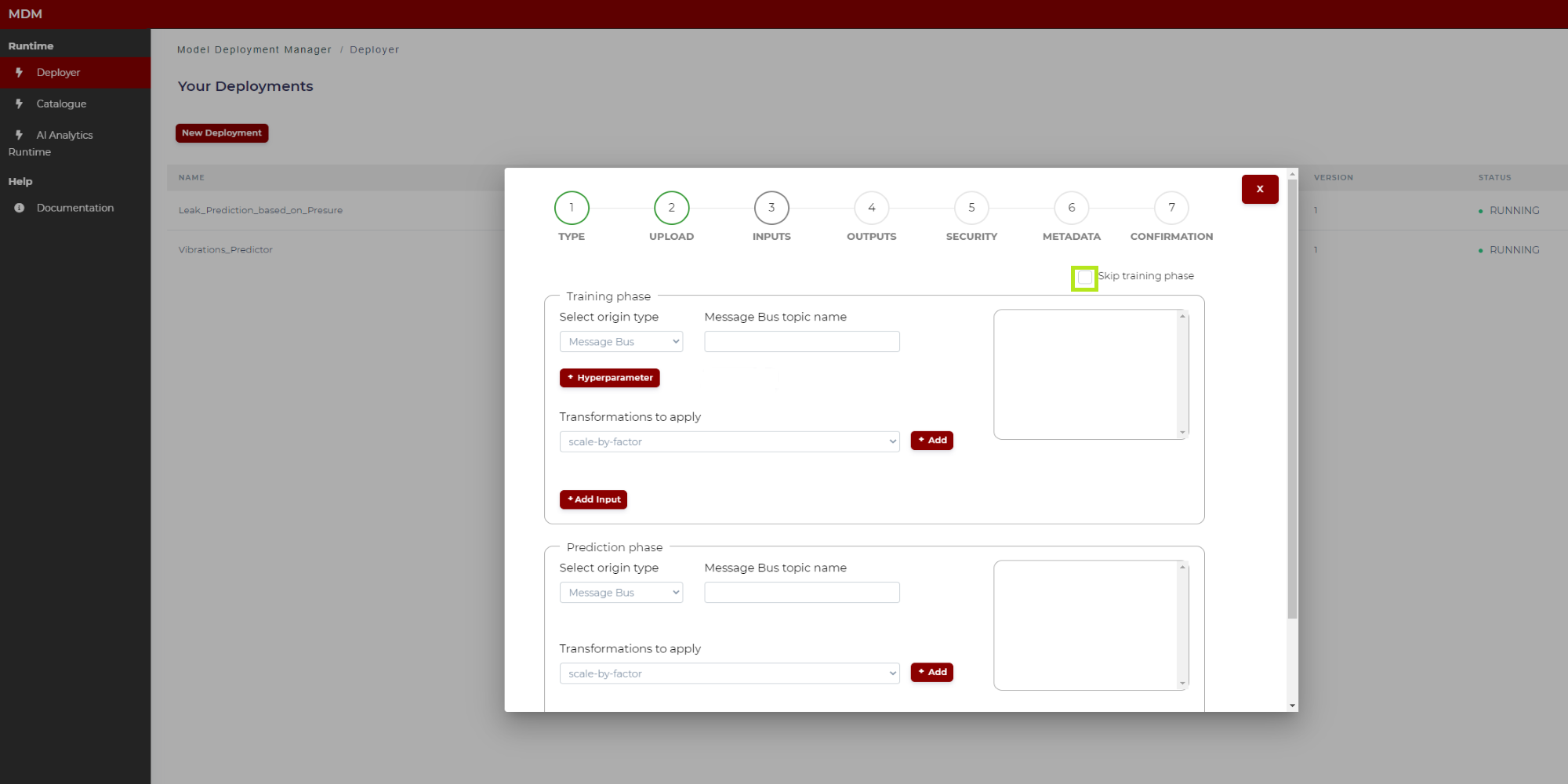
Figure 10. Input signals specification
Training phase
In Figure 11, the different steps of the training phase configuration have been marked and numbered.
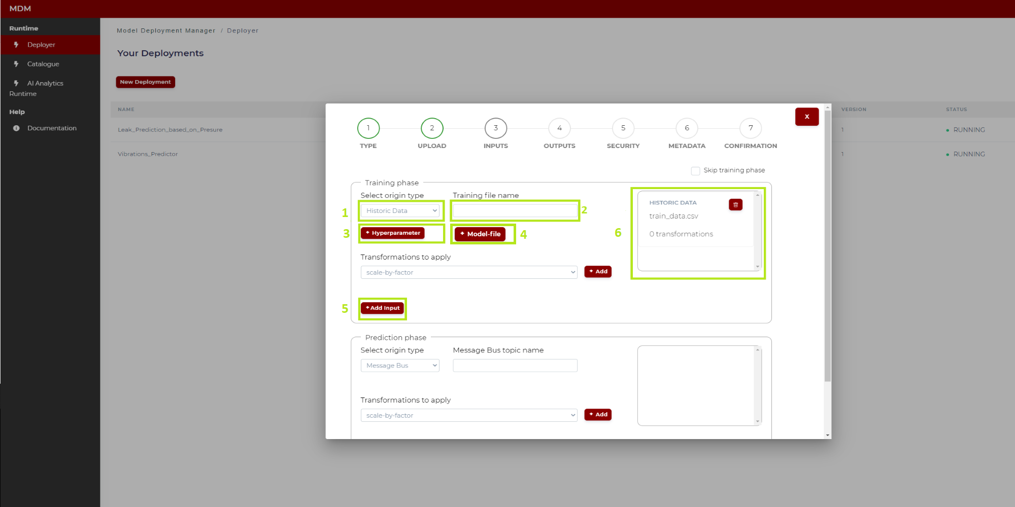
Figure 11. Training phase configuration
Below are the instructions to configure the training phase:
1: To select the origin type of the input data, the user clicks on the drop down and selects one of the two available options: “Historic data” or “Message Bus”. The following instructions indicate the steps in case the user selects the origin type “Historic data”
2: Once the user has selected in 1 “Historic data”, in the field “Training file name” the user types the name of the CSV file containing the dataset that will be used in the training process, which will be the first operation run in the AI Analytics Run-time after completion of the deployment steps described here. By that time, this file will need to be uploaded in the Storage of the AI Analytics Run-time as shown in Figure 12: click on “Storage” (in the side menu on the left), and then click on “Upload new dataset”
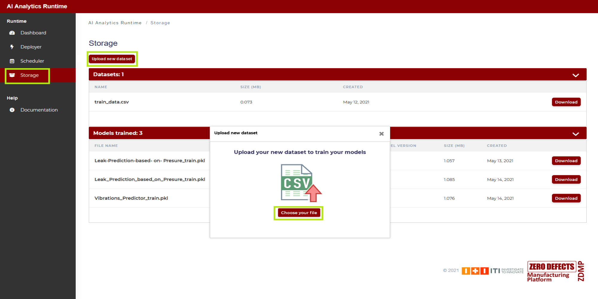
Figure 12. Uploading a dataset file to AI Analytics Run-time Storage area
3: The “Hyperparameters” are parameters specific of the selected machine learning algorithms to be used in the training process. If needed, clicking on this button, a pop-up window appears allowing the user to type the hyperparameters list in JSON format
4: Clicking on the “Model file“ button, a pop-up windows appears allowing the user to type the name of the model file (for example trained_model.pkl) which will be generated by the training process and saved in the models area of the AI Analytics Run-time Storage. In case the “src” folder already includes a pkl file corresponding to a trained model, as described in section “Step 2: Upload the model”, then the user does not need to fill in the field “Model file” as the name of the pkl file is automatically detected and included in the manifest
5: Finally, the user clicks on “Add input” and this training input is fully configured
6: When this training input is fully configured is added to a list on the right side of the screen. The user can delete the configured input if needed
In case the origin type of the training input is “Message Bus” instead of “Historic data”, the configuration must follow the same steps indicated in the following section for the prediction phase. Note that this might be the case when the selected algorithm implements a continuous (incremental or adaptive) learning approach, as is the case for some of the machine learning described in the final sections.
Prediction phase with origin type Message Bus
To explain it better, in the following image the training phase has been skipped and the various parts of the screen have been marked and numbered in green:
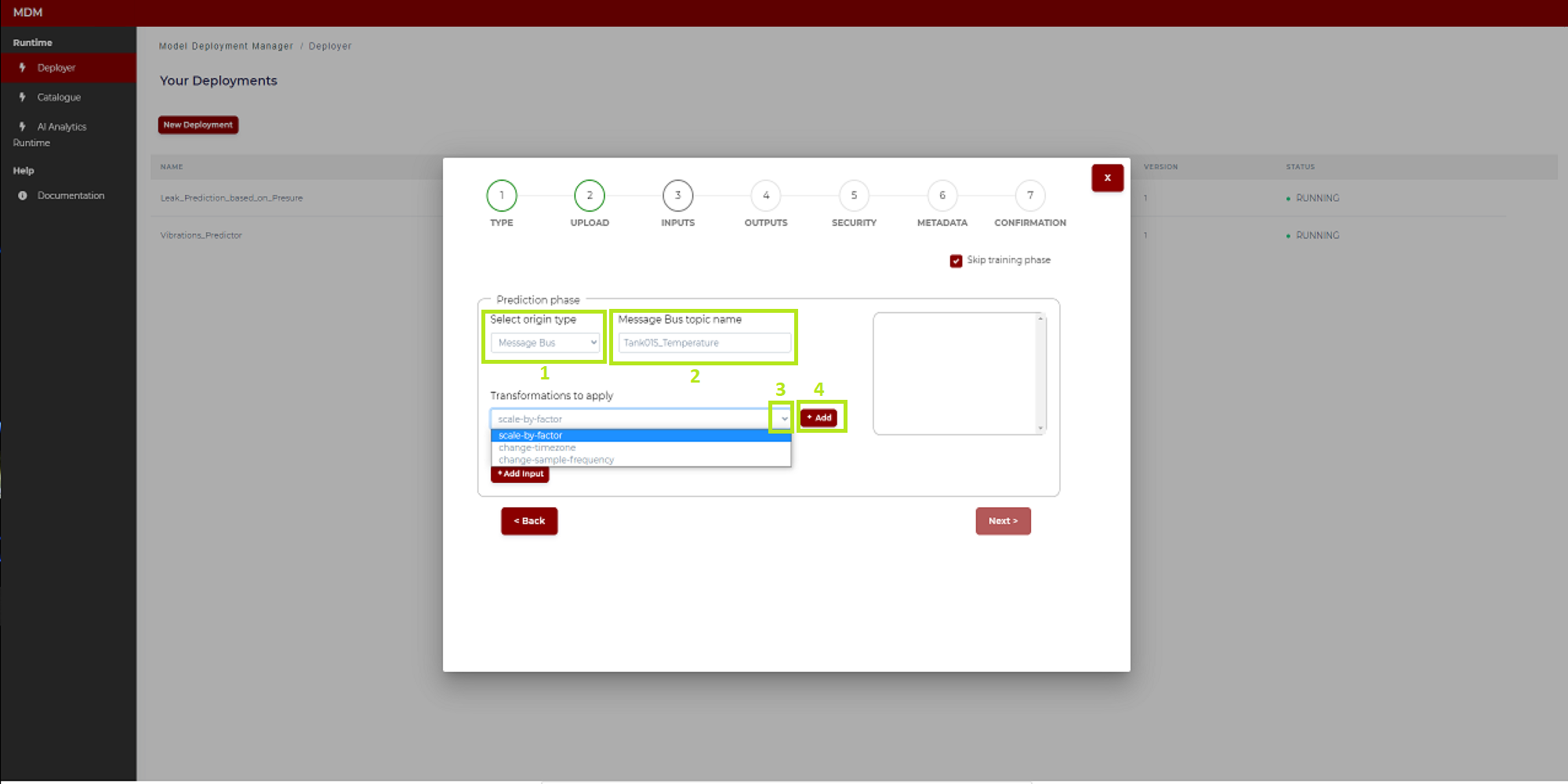
Figure 13. Prediction phase configuration with origin type Message Bus
These are the instructions to configure an input signal:
1: To select the origin type of the input, Click on the tab. The user can select between two origin types: “Message Bus” or “Rest API”. As the title of this subsection indicates, here is explained the case of origin type “Message Bus”
2: In the field “Message Bus topic name” the user types the corresponding topic
3: In the section “Transformations to apply” the user clicks on the tab and a drop-down menu opens with the different transformations available in the Data Processor
4: Clicking on the “Add” button, the transformation selected in “3” appears in a table. In case of selecting, for example, the transformation “scale by factor”, then the screen is as shown in the figure below
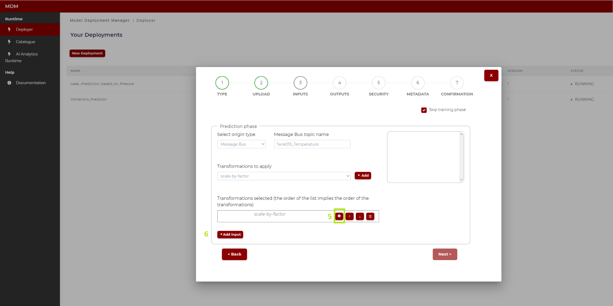
Figure 14. Example of transformation (“scale by factor”)
5: Clicking on the “settings” symbol the user configures this transformation. The configuration of each of the transformations available in the Data Processor is explained in the following sub-section “Configuring Data Processor transformations”
6: When the user has finished loading and configuring all the transformations to be applied to this input signal, then the user can click on “Add input” and this input signal is fully configured
7: When the input signal is fully configured, it is added to a list on the right side of the screen as shown in Figure 15. The user can delete this configured input if needed
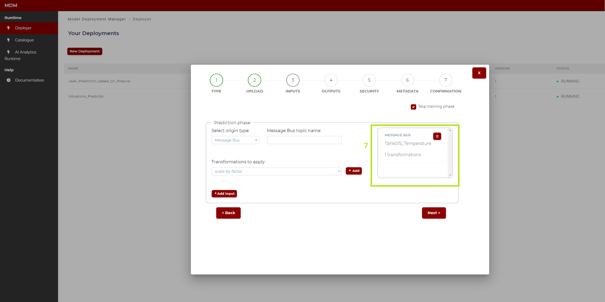
Figure 15. Input signal configuration
At this point, the user can select another input signal and repeat the process until all the input signals needed are configured.
Prediction phase with origin type Rest API
If the origin type of the input is “Rest API” the Prediction phase section is as shown in Figure 16:
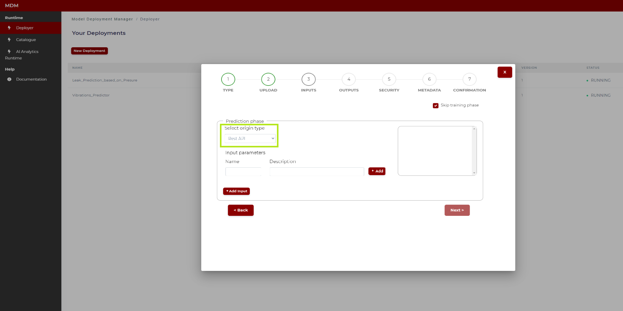
Figure 16. Prediction phase with origin type Rest API (before configuration)
In Figure 17 the various parts of the screen have been marked and numbered in green to explain the configuration steps:
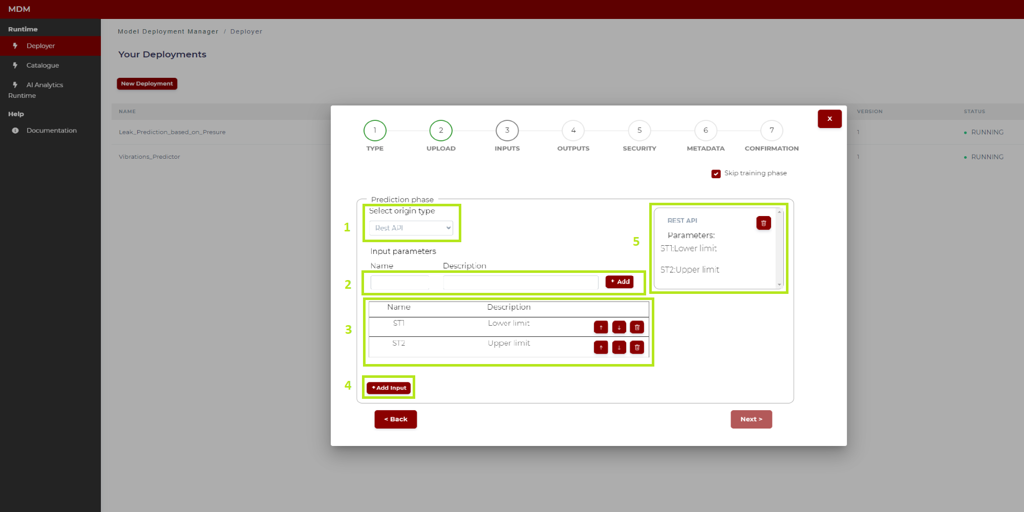
Figure 17. Prediction phase with origin type Rest API (after configuration)
1: The user selects origin type “Rest API”
2: The user types the “Name” and “Description” of a parameter, then click on “Add” and this parameter is added in the list “3”
3: All parameters added in “2” are shown in this list. The user can change the order in the list by clicking on the arrows up/down, and also can delete a row if needed
4: When all the parameters have been added to the list, the user clicks on “Add input” and the Rest API input is fully configured
5: When the Rest API is fully configured, it is added on the right side of screen. The user can delete it if needed
Configuring Data Processor transformations
This section describes how to configure the different transformations available at the moment in the Data Processor. In the next stage of the project, it is expected that more data transformations will be available such as mean centring, z-score normalization, and missing data.
When configuring inputs and outputs, if needed, the user can configure data transformations. As shown in Figure 18 the user selects the data transformation in the drop-down, clicks on “Add” to add it to the list, and then clicks on the “setting” symbol to configure this transformation.
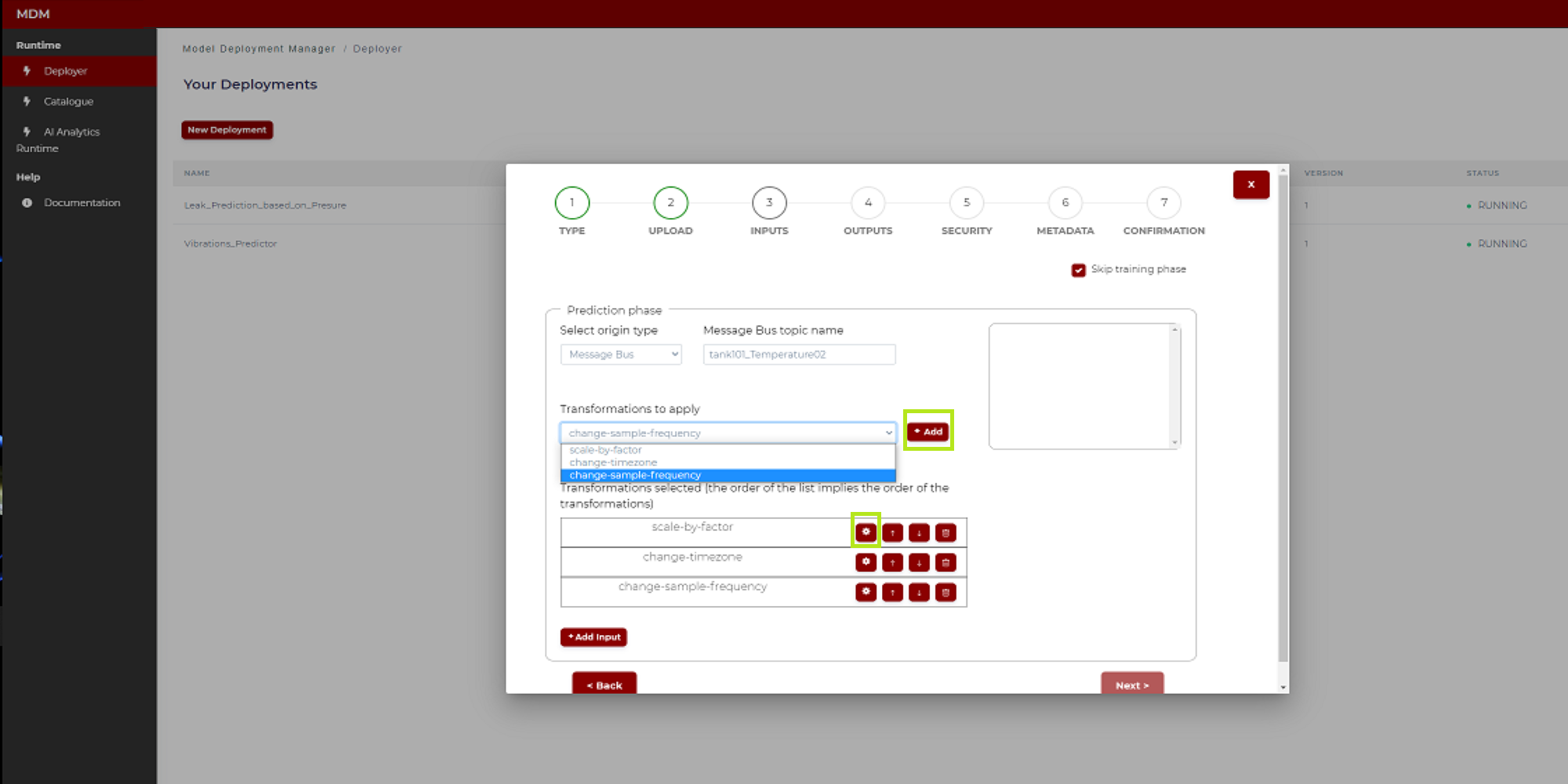
Figure 18. Data transformations
Each of the available transformations are described below:
- Scale by factor: The values of the signal are multiplied by a factor introduced by user. It is used in conversions of units of measure or scaling data to fit into the appropriate format/range. Clicking on the “setting” symbol a pop-up window appears as shown in the following image. The user only has to type the factor (a real number with comma separated decimals)
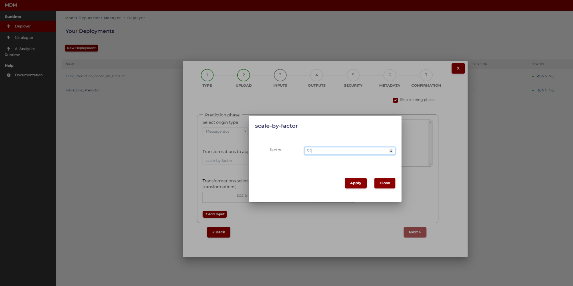
Figure 19. Example of scale by factor transformation
- Change time zone: It is used when data collected from different time zones need to be aligned. The user selects the origin time zone and the target time zone. The timestamps of the signal (which was collected in the origin time zone) will be changed from origin time zone to target time zone. The following image shows how the user chooses the time zones by selecting from a drop-down list that includes all the time zones in the world
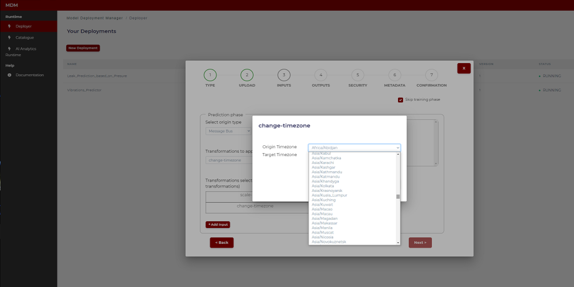
Figure 20. Example of time zone change transformation
- Change sample frequency: This transformation is used when data collected with different sample frequencies need to have the same frequency. The user only has to introduce the time period between samples. As shown in the image below there is a field to enter a numeric value and another to select the time unit (second, minute, hour, etc)
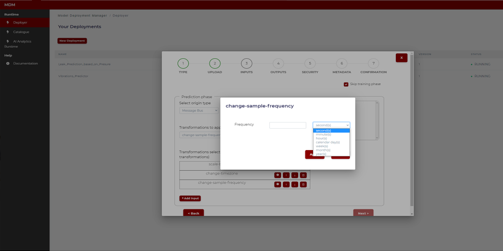
Figure 21. Example of sample frequency transformation
Step 4: Outputs
In this step the user configures the output signals where the model will write the results. For both prediction and training phases, the only possible destination type is “Message Bus”. To configure the outputs, follow the same steps indicated in section “Prediction phase with origin type Message Bus” and in case transformations are needed on the outputs, proceed as explained in section “Configuring Data Processor transformations”. The results will be published to all the given topics: if it is a prediction message bus topic, new predictions made for each input received will be published, while if it is a training message bus topic, once the training is finished, the model file will be saved, and the training statistics will be published.
Step 5: Security
The user selects which roles, previously defined in the platform by the user responsible of managing the company profiles, will have access to the model once deployed: Only users owing the selected roles will be allowed to access.
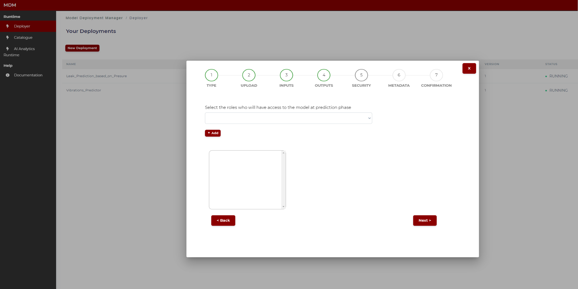
Figure 22. Specifying model security
Step 6: Metadata
The user types the following fields, which are necessary to construct the manifest:
Name: Name of the model
Version: Version of the model (format must be x.y.z)
Tags: Tags separated by commas which will be associated to the model. These tags will be used to apply filters
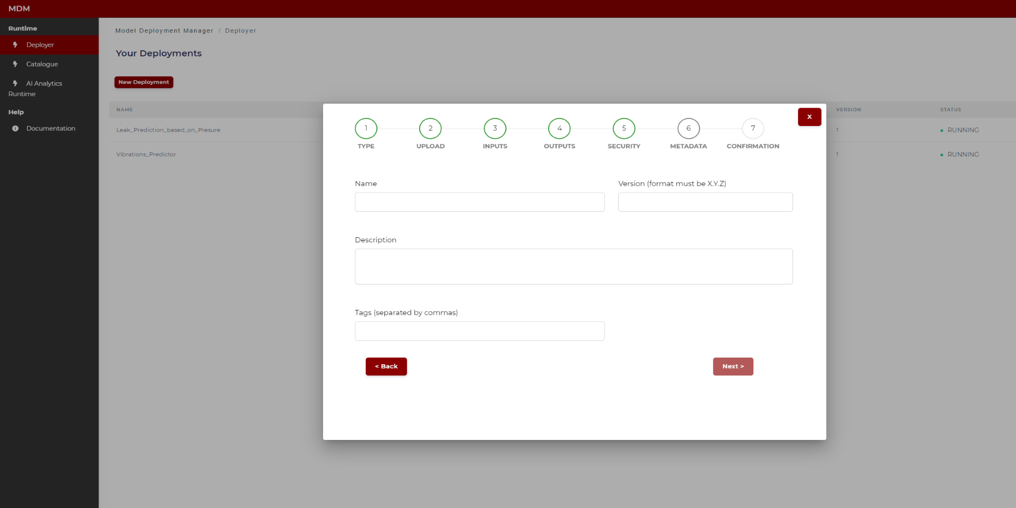
Figure 23. Specifying model metadata
Step 7: Confirmation
This is the last step in the wizard. The user can see in the screen the manifest to review if the data collected through different steps are correct. By clicking on “Save” this manifest JSON file together with the model is sent to the AI Analytics Run-time, which after a few moments, automatically will deploy the model for run time.
The figures below show the top of the manifest and the bottom (when the user moves the scroll through the window).
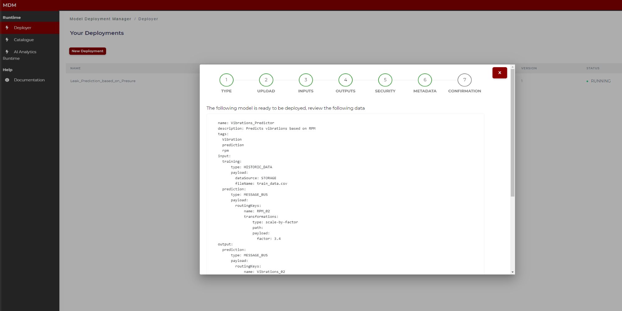
Figure 24. Final manifest example (top)
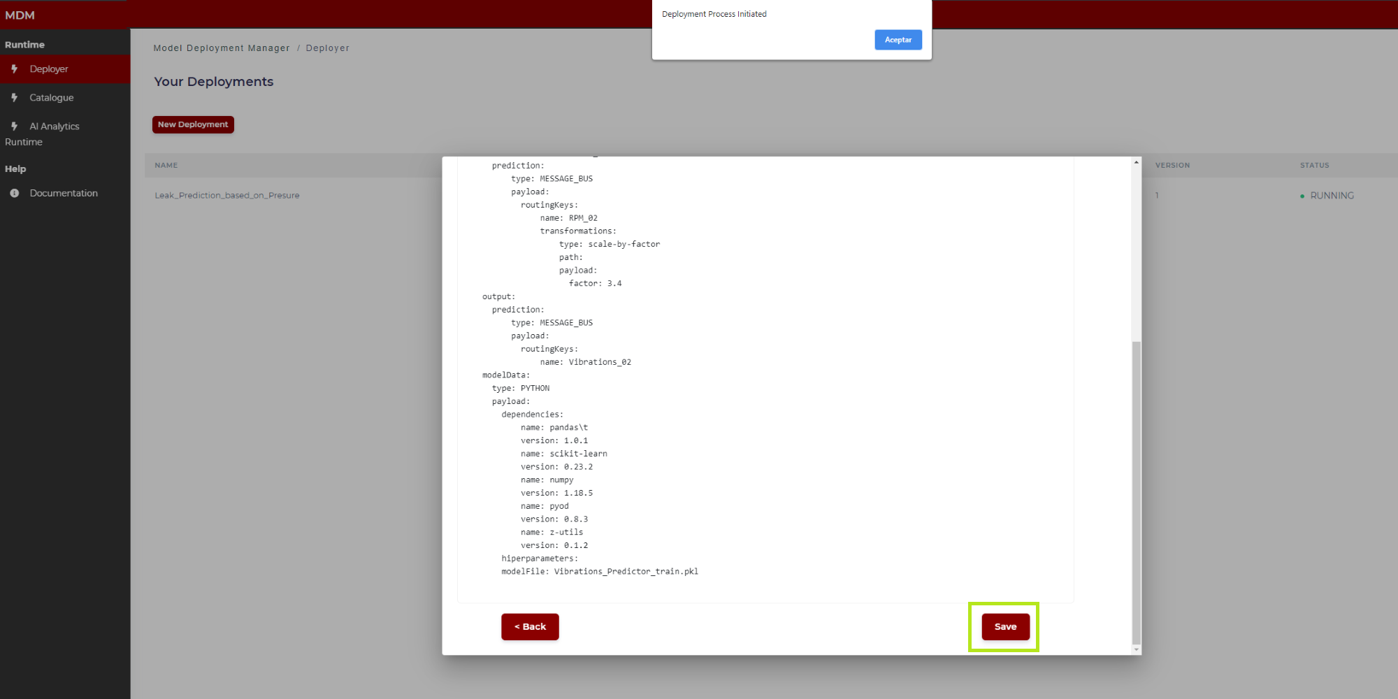
Figure 25. Final manifest example (bottom)
General Considerations
For ease of use and to the structure defined for the Model Deployment Manager, all the algorithms have been packaged into two main files, one for training (“train.py”) and another one for prediction (“predict.py”).
For all the algorithms, there is an example of use of both “train.py” and “predict.py” functions in the “example.py” file in the source code folder.
Unsupervised Anomaly Detection
Principal Component Analysis (PCA)
Description
Principal Component Analysis (PCA) is a technique for Unsupervised Anomaly Detection which involves decomposing the covariance matrix into eigenvalues, usually after scaling the variables to zero mean and unit variance. This transformation allows a new coordinate system to be constructed for the original data set in which the largest variance of the data set is captured on the first axis, the second largest variance is the second axis etc. Each of these axes is called principal component or latent variable.
PCA is often used as a dimensionality reduction technique, allowing the original data to be compressed into a few latent variables (principal components) and then reconstructing the data from those latent variables.
The PCA has two statistics to determine the anomaly score in the data: Squared Prediction Error (SPE) and Hotelling’s T2. Each of these statistics has its own control limit or UCL (Upper Control Limit) that allows knowing if an observation is anomalous or not.
Apart from the ability to detect anomalies, the PCA has the contribution graphs (either from the SPE or from Hotelling’s T2), which allow to know the causes of such anomalies. This ability to diagnose the anomaly is unique to the PCA and is not found in any other anomaly detection method. This is a particularly important characteristic when it comes to better understanding the data under study, that is, better understanding the mechanisms that have caused the anomalies.
The developed library provides the following features:
Implemented algorithms: Singular Value Decomposition (SVD) and NIPALS (Nonlinear Iterative Partial Least Squares):
With SVD all the components must be calculated even though the higher ones are not needed
NIPALS computes the components iteratively
SVD is faster for small datasets and NIPALS is more suitable for large datasets. The implemented algorithms cannot manage missing values
Automatic number of components computation; either:
Able to specify a determined number of components by user
Class will compute the optimal number of components automatically by cross validation
Class will compute the number of components that explain a determined R2 value specified by the user
Data cleansing: Create a function to obtain Normal Operating Conditions for a given dataset, by removing outliers. Possibilities implemented:
To remove the more extreme observations (those with values greater than 3 times the upper control limits). Able to specify a determined number of components by user
To perform a deeper cleansing, by removing the observations with higher values of the statistics (SPE and Hotelling’s T2) until having a 5% of out-of-control observations (which is the statistically expected percentage)
Fault detection: Compute SPE and T² Hotelling’s statistics and its corresponding Upper Control Limits to detect abnormal situations
Fault diagnosis: Compute contributions to SPE and T² Hotelling’s to identify which features are responsible of such abnormal situations
Training
The parameters of the training function are the following:
json_data (string): A JSON with data to train
s_model (string): The path where the model will be stored
predictors (list, optional, default=None): The list of variables to consider for model training
n_components (integer, optional, default=-1):
If -1 the components will be computed automatically.
If >0 the model will be fit with n_components
n_comp_criteria (float or string, optional, default=0.9): Criteria for the selection of the number of components:
If it is a number between [0,1] it specifies the minimum value of R2 that the model must achieve. That is, the model must have the minimum number of components that give the specified value of R2
If it is “Q2” then the number of components will be computed automatically by cross-validation based on Q2 trend
scale (boolean, optional default=True): Whether to scale the data or not. By default, data is standardized to unit variance and zero‑mean
cleansing (string, optional, default=‘none’): Must be one of the following:
‘none’: No data cleansing is done at all
‘extreme’: Remove observations with SPE (or T2) greater than 3*UCL
‘full’: Remove observations with SPE (or T2) greater than 3*UCL and remove highest values in SPE (or T2) until having a 5% of out-of-control observations
algorithm (string, optional, default=‘SVD’): Algorithm to compute PCA. Must be one of the following:
‘SVD’: Singular Value Decomposition
‘NIPALS’: Nonlinear Iterative Partial Least Squares
Note: with SVD all the components must be calculated even though the higher ones are not needed, while NIPALS computes the components iteratively. SVD is usually faster for little datasets and NIPALS is more suitable for large datasets
tol_variance_filter (float, optional, default=1e-05): Removes features with coefficient of variation less than tol_variance_filter. This avoids problems with constant features or features with low variance which are not useful for the model.
When fitting the PCA model the SPE (Squared prediction error) and the Hotelling’s T² statistics are computed. The corresponding upper control limits (UCL) of both statistics are also computed. All this information is stored as properties in the PCA model object.
The training function returns two values:
List that contains error info if any error occurs, null otherwise
R2 of the predictions
Predict
Once the model is trained, predictions can be obtained using the “predict.py” module that has the following parameters:
json_data (string): A JSON with data to predict
s_model (string): The path where the model is stored
The results of the prediction function are a JSON with the following structure:
“result”: predicted value with the possible values ‘Under control’, ‘Anomaly (SPE)’, ‘Anomaly (T2)’ or ‘Anomaly (SPE+T2)’
“payload”: contains the following fields:
“UCL_SPE”: Upper Control Limit for Squared Prediction Error
“SPE”: Value of Squared Prediction Error statistic
“SPE_contrib”: Dictionary with SPE contributions (one per variable)
“UCL_T2”: Upper Control Limit for T2 Hotelling’s statistic
“T2”: Value of T2 Hotelling’s statistic
“T2_contrib”: Dictionary with T2 contributions (one per variable)
PCA is able to detect abnormal situations but to know which are the features that are responsible of such abnormalities. When the observation is an anomaly, it could be because the SPE statistic is above UCL_SPE and/or because T2 is above UCL_T2. Then the corresponding contributions (SPE_contrib and/or T2_contrib) should be checked. As stated before, contributions are given as a dictionary where the key is the name of the variable, and the value is the contribution of that variable. Variables with higher contributions should be investigated to find the root causes of the anomaly.
PCA (online)
This is an extension of the Principal Component Analysis algorithm to work in online mode. To achieve this, a sliding window technique will be used. Two parameters will be incorporated: the frequency (number of instances) to update the model and the size of the window to use for such update. So, the parameters of the training function of the PCA online are the same as in Principal Component Analysis (PCA) plus additional parameters:
n_update_freq (integer, optional, default=100): Training frequency, that is, the model will be trained after “n_update_freq” instances
n_update_size (integer, optional, default=500): The model will be trained with the last “n_update_size” instances
Autoencoder
Description
Autoencoder is a technique for Unsupervised Anomaly Detection. Autoencoders are a dimensionality reduction technique so they can be considered an alternative to PCA (Principal Component Analysis) when nonlinearities are present. The hidden layer has a much smaller number of nodes than the input layer, so the output nodes of this hidden layer can be interpreted as a reduced representation of the data. Certain simplified Autoencoder architectures have been shown to result in a reduction in dimensionality similar to that achieved with PCA. The architecture on both sides of the hidden layer is usually symmetrical. In fact, the Autoencoder can be divided into two parts on either side of the middle layer called encoder and decoder. That is to say, the Autoencoder is capable of compressing the data (encoder) and then reconstructing it (decoder). As with the PCA, the Autoencoder captures the information from most observations, which are normal observations, so when reconstructing the data, anomalous observations will have a much greater error than normal observations. This error can be used as a measure of the degree of anomaly of the observations. The implemented library is a wrapper of the Autoencoder’s PyOD library.
Training
The parameters of the training function are the following:
json_data (string): A JSON with data to train
s_model (string): The path where the model will be stored
predictors (list, optional, default=None): The list of variables to consider for model training
categoricals: (list, optional, default=None): The list of categorical variables
hidden_neurons (list, optional, default= [64, 32, 32, 64]): The number of neurons per hidden layers
hidden_activation (string, optional, default=‘relu’): Activation function to use for hidden layers. All hidden layers are forced to use the same type of activation. See https://keras.io/activations/
output_activation: (string, optional, default=‘sigmoid’): Activation function to use for output layer. See https://keras.io/activations/
loss (string or obj, optional, default=keras.losses.mean_squared_error): String (name of objective function) or objective function. See https://keras.io/losses/
optimizer (string, optional, default=‘adam’): String (name of optimizer) or optimizer instance. See https://keras.io/optimizers/
epochs: (integer, optional, default=100): Number of epochs to train the model
batch_size (integer, optional, default=32): Number of samples per gradient update
dropout_rate (float in (0, 1), optional, default=0.2): The dropout to be used across all layers
l2_regularizer (float in (0., 1), optional, default=0.1): The regularization strength of activity_regularizer applied on each layer. By default, l2 regularizer is used. See https://keras.io/regularizers/
validation_size (float in (0., 1), optional, default=0.1): The percentage of data to be used for validation
contamination (float in (0., 0.5), optional, default=0.1): The amount of contamination of the data set, ie the proportion of outliers in the data set. When fitting this is used to define the threshold on the decision function
The training function returns a list that contains error info if any error occurs, null otherwise.
Predict
Once the model is trained, predictions can be obtained using the “predict.py” module that has the following parameters:
json_data (string): A JSON with data to predict
s_model (string): The path where the model is stored
The results of the prediction function are a JSON with the following structure:
“label”: Predicted values (0-inlier,1-outlier)
“score”: Anomaly score
“limit”: Upper threshold. Scores above this limit are considered outliers (anomalies)
Autoencoder (online)
This is an extension of the Autoencoder algorithm to work in online mode. To achieve this, a sliding window technique will be used. Two parameters will be incorporated: the frequency (number of instances) to update the model and the size of the window to use for such update. So, the parameters of the training function of the Autoencoder online are the same as in Autoencoder plus additional parameters:
n_update_freq (integer, optional, default=100): Training frequency, that is, the model will be trained after “n_update_freq” instances
n_update_size (integer, optional, default=500): The model will be trained with the last “n_update_size” instances
Isolation Forest
Description
Isolation Forest is a technique for Unsupervised Anomaly Detection. An Isolation Forest is an ensemble (combination) of a series of isolation trees. In an isolation tree, data is recursively partitioned by cuts parallel to the axes at cut-off points that are selected randomly and in dimensions (variables) also selected randomly. The process repeats until each node contains a single instance. The branches that contain the anomalies are shallower since the anomalous data are found in more dispersed regions than the normal data, so they are more easily separable from the rest of the observations. Therefore, the distance between the end node and the root node is used as a measure of the degree of anomaly. The definitive degree of anomaly is obtained by averaging the lengths of the branches of the observations in the different trees of the Isolation Forest. The implemented library is a wrapper of the Isolation Forest’s PyOD library.
Training
The parameters of the training function are the following:
json_data (string): A JSON with data to train
s_model (string): The path where the model will be stored
predictors (list, optional, default=None): The list of variables to consider for model training
categoricals: (list, optional, default=None): The list of categorical variables
n_estimators (integer, optional, default=100): The number of base estimators in the ensemble
max_samples (integer or float, optional, default=“auto”): The number of samples to draw from X to train each base estimator:
If integer, then draw max_samples samples
If float, then draw max_samples * X.shape[0] samples
If “auto”, then max_samples=min(256, n_samples)
If max_samples is larger than the number of samples provided, all samples will be used for all trees (no sampling)
contamination (float in (0., 0.5), optional, default=0.1): The amount of contamination of the data set, ie the proportion of outliers in the data set. Used when fitting to define the threshold on the decision function
max_features (integer or float, optional, default=1.0): The number of features to draw from X to train each base estimator:
If integer, then draw max_features features
If float, then draw max_features * X.shape[1] features
bootstrap (boolean, optional, default=False): If True, individual trees are fit on random subsets of the training data sampled with replacement. If False, sampling without replacement is performed
The training function returns a list that contains error info if any error occurs, null otherwise.
Predict
Once the model is trained, predictions can be obtained using the “predict.py” module that has the following parameters:
json_data (string): A JSON with data to predict
s_model (string): The path where the model is stored
The results of the prediction function are a JSON with the following structure:
“label”: Predicted values (0-inlier,1-outlier)
“score”: Anomaly score
“limit”: Upper threshold. Scores above this limit are considered outliers (anomalies)
Isolation Forest ASD
Description
Isolation Forest is an efficient method for anomaly detection with relatively low complexity, CPU, and time consumption. It requires all the data in the beginning to build t random samples. It also needs many passes over the dataset to build all the random forest. So, it is not adapted to data stream context. To overcome these drawbacks, the so-called Isolation Forest Algorithm for Stream Data (IForestASD) method has been proposed which is an improvement of IForest for anomaly detection in data streams. IForestASD uses sliding window to deal with streaming data. On the current complete window, IForestASD executes the standard IForest method to get the random forest. This is the IForest detector model for IForestASD. IForestASD method can also deal with concept drift in the data stream by maintaining one input desired anomaly rate (u). If the anomaly rate in the considered window is upper than u, then a concept drift occurred so IForestASD deletes its current IForest detector and builds another one using all the data in the considered window. The implemented library is a wrapper of the Isolation Forest ASD’s PySAD library.
Training
The parameters of the training function are the following:
json_data (string): A JSON with data to train
s_model (string): The path where the model will be stored
predictors (list, optional, default=None): The list of variables to consider for model training
categoricals: (integer, optional, default=100): The list of categorical variables
n_initial_fit (integer, optional, default = 5): Number of instances for an initial training. The model will be trained for the first time after this number of instances. Predictions will not be available during this initial period
window_size (integer, optional, default=2048): The size of the reference window and its sliding
contamination (float in (0., 0.5), optional, default=0.1): The amount of contamination of the data set, ie the proportion of outliers in the data set. When fitting this is used to define the threshold on the decision function
The training function returns a list that contains error info if any error occurs, null otherwise.
Predict
Once the model is trained, predictions can be obtained using the “predict.py” module that has the following parameters:
json_data (string): A JSON with data to predict
s_model (string): The path where the model is stored
The results of the prediction function are a JSON with the following structure:
“label”: Predicted values (0-inlier,1-outlier)
“score”: Anomaly score
“limit”: Upper threshold. Scores above this limit are considered outliers (anomalies)
KitNet
Description
KitNET is a lightweight online anomaly detection algorithm based on an ensemble of autoencoders. Each autoencoder in the ensemble is responsible for detecting anomalies relating to a specific aspect of the process behaviour. KitNet is designed to run on simple machines and in real-time, so it has been designed with small memory footprint and a low computational complexity. The implemented library is a wrapper of the KitNet’s PySAD library.
Training
The parameters of the training function are the following:
json_data (string): A JSON with data to train
s_model (string): The path where the model will be stored
predictors (list, optional, default=None): The list of variables to consider for model training
categoricals: (list, optional, default=None): The list of categorical variables
n_initial_fit (integer, optional, default=100): Number of instances for an initial training. The model will be trained for the first time after this number of instances. Predictions will not be available during this initial period
contamination (float in (0., 0.5), optional, default=0.1): The amount of contamination of the data set, ie the proportion of outliers in the data set. When fitting this is used to define the threshold on the decision function
max_size_ae (integer, optional, default=10): The maximum size of any autoencoder in the ensemble layer
learning_rate (float in (0, 1), optional, default=0.1): The default stochastic gradient descent learning rate for all autoencoders in the KitNET instance
hidden_ratio (float in (0, 1), optional, default=0.75): The default ratio of hidden to visible neurons. E.g., 0.75 will cause roughly a 25% compression in the hidden layer
The training function returns a list that contains error info if any error occurs, null otherwise.
Predict
Once the model is trained, predictions can be obtained using the “predict.py” module that has the following parameters:
json_data (string): A JSON with data to predict
s_model (string): The path where the model is stored
The results of the prediction function are a JSON with the following structure:
“label”: Predicted values (0-inlier,1-outlier)
“score”: Anomaly score
“limit”: Upper threshold. Scores above this limit are considered outliers (anomalies)
K-Nearest Neighbour (KNN)
Description
KNN is a technique for Unsupervised Anomaly Detection. In this case the degree of anomaly of an observation is based on the distance to the k‑th nearest neighbour. The implemented library is a wrapper of the KNN’s PyOD library.
Training
The parameters of the training function are the following:
json_data (string): A JSON with data to train
s_model (string): The path where the model will be stored
predictors (list, optional, default=None): The list of variables to consider for model training
categoricals: (list, optional, default=None): The list of categorical variables
n_neighbors (integer, optional, default = 5): Number of neighbours to use by default for k neighbours queries
method (string, optional, default=‘largest’). Must be one of the following:
‘largest’: Use the distance to the kth neighbour as the outlier score
mean’: Use the average of all k neighbours as the outlier score
‘median’: Use the median of the distance to k neighbours as the outlier score
radius (float, optional, default = 1.0): Range of parameter space to use by default for `radius_neighbors` queries
algorithm (string, optional, default=’auto’). Algorithm used to compute the nearest neighbours. Must be one of the following:
‘ball_tree’ will use BallTree
‘kd_tree’ will use KDTree
‘brute’ will use a brute-force search
‘auto’ will attempt to decide the most appropriate algorithm based on the values passed to fit method
leaf_size (integer, optional, default = 30): Leaf size passed to BallTree. This can affect the speed of the construction and query, as well as the memory required to store the tree. The optimal value depends on the nature of the problem
metric (string or callable, default ‘minkowski’): Metric to use for distance computation. Any metric from scikit-learn or scipy.spatial.distance can be used. If metric is a callable function, it is called on each pair of instances (rows) and the resulting value recorded. The callable should take two arrays as input and return one value indicating the distance between them. This works for Scipy’s metrics but is less efficient than passing the metric name as a string. Distance matrices are not supported. Valid values for metric are (see the documentation for scipy.spatial.distance for details on these metrics:
from scikit-learn: [‘cityblock’, ‘cosine’, ‘euclidean’, ‘l1’, ‘l2’, ‘manhattan’]
from scipy.spatial.distance: [‘braycurtis’, ‘canberra’, ‘chebyshev’, ‘correlation’, ‘dice’, ‘hamming’, ‘jaccard’, ‘kulsinski’, ‘mahalanobis’, ‘matching’, ‘minkowski’, ‘rogerstanimoto’, ‘russellrao’, ‘seuclidean’, ‘sokalmichener’, ‘sokalsneath’, ‘sqeuclidean’, ‘yule’]
p (integer, optional, default = 2): Parameter for the Minkowski metric from scikit-learn.metrics.pairwise.pairwise_distances. When p = 1, this is equivalent to using manhattan_distance (l1), and euclidean_distance (l2) for p = 2. For arbitrary p, minkowski_distance (l_p) is used. See http://scikit-learn.org/stable/modules/generated/scikit-learn.metrics.pairwise.pairwise_distances
metric_params (dict, optional, default = None): Additional keyword arguments for the metric function
contamination (float in (0., 0.5), optional, default=0.1): The amount of contamination of the data set, ie the proportion of outliers in the data set. When fitting this is used to define the threshold on the decision function
The training function returns a list that contains error info if any error occurs, null otherwise.
Predict
Once the model is trained, predictions can be obtained using the “predict.py” module that has the following parameters:
json_data (string): A JSON with data to predict
s_model (string): The path where the model is stored
The results of the prediction function are a JSON with the following structure:
“label”: Predicted values (0-inlier,1-outlier)
“score”: Anomaly score
“limit”: Upper threshold. Scores above this limit are considered outliers (anomalies)
KNN (online)
This is an extension of the K-Nearest Neighbour algorithm to work in online mode. To achieve this, a sliding window technique will be used. Two parameters will be incorporated: the frequency (number of instances) to update the model and the size of the window to use for such update. So, the parameters of the training function of the KNN online are the same as in K-Nearest Neighbour (KNN) plus two more additional parameters:
n_update_freq (integer, optional, default=100): Training frequency, that is, the model will be trained after “n_update_freq” instances
n_update_size (integer, optional, default=500): The model will be trained with the last “n_update_size” instances
Local Outlier Factor (LOF)
Description
Local Outlier Factor (LOF) is a technique for Unsupervised Anomaly Detection which measures the local deviation of density of a given sample with respect to its neighbours. It is local in that the anomaly score depends on how isolated the object is with respect to the surrounding neighbourhood. More precisely, locality is given by k-nearest neighbours, whose distance is used to estimate the local density. By comparing the local density of a sample to the local densities of its neighbours, one can identify samples that have a substantially lower density than their neighbours. These are considered outliers. The implemented library is a wrapper of the LOF’s PyOD library.
Training
The parameters of the training function are the following:
json_data (string): A JSON with data to train
s_model (string): The path where the model will be stored
predictors (list, optional, default=None): The list of variables to consider for model training
categoricals: (list, optional, default=None): The list of categorical variables
n_neighbors (integer, optional, default=20): Number of neighbours to use by default for `kneighbors` queries. If n_neighbors is larger than the number of samples provided, all samples will be used
algorithm (string, optional, default=’auto’). Algorithm used to compute the nearest neighbours. Must be one of the following:
‘ball_tree’ will use BallTree
‘kd_tree’ will use KDTree
‘brute’ will use a brute-force search
‘auto’ will attempt to decide the most appropriate algorithm based on the values passed to fit method
leaf_size (integer, optional, default=30): Leaf size passed to `BallTree` or `KDTree`. This can affect the speed of the construction and query, as well as the memory required to store the tree. The optimal value depends on the nature of the problem
metric (string or callable, default ‘minkowski’): Metric used for the distance computation. Any metric from scikit-learn or scipy.spatial.distance can be used. If ‘precomputed’, the training input X is expected to be a distance matrix. If metric is a callable function, it is called on each pair of instances (rows) and the resulting value recorded. The callable should take two arrays as input and return one value indicating the distance between them. This works for Scipy’s metrics but is less efficient than passing the metric name as a string. Valid values for metric are (See the documentation for scipy.spatial.distance for details on these metrics: http://docs.scipy.org/doc/scipy/reference/spatial.distance.html):
from scikit-learn: [‘cityblock’, ‘cosine’, ‘euclidean’, ‘l1’, ‘l2’, ‘manhattan’]
from scipy.spatial.distance: [‘braycurtis’, ‘canberra’, ‘chebyshev’, ‘correlation’, ‘dice’, ‘hamming’, ‘jaccard’, ‘kulsinski’, ‘mahalanobis’, ‘matching’, ‘minkowski’, ‘rogerstanimoto’, ‘russellrao’, ‘seuclidean’, ‘sokalmichener’, ‘sokalsneath’, ‘sqeuclidean’, ‘yule’]
p (integer, optional, default = 2): Parameter for the Minkowski metric from scikit-learn.metrics.pairwise.pairwise_distances. When p = 1, this is equivalent to using manhattan_distance (l1), and euclidean_distance (l2) for p = 2. For arbitrary p, minkowski_distance (l_p) is used. See http://scikit-learn.org/stable/modules/generated/scikit-learn.metrics.pairwise.pairwise_distances
metric_params (dictionary, optional, default = None): Additional keyword arguments for the metric function
contamination (float in (0., 0.5), optional, default=0.1): The amount of contamination of the data set, ie the proportion of outliers in the data set. When fitting this is used to define the threshold on the decision function
The training function returns a list that contains error info if any error occurs, null otherwise.
Predict
Once the model is trained, predictions can be obtained using the “predict.py” module that has the following parameters:
json_data (string): A JSON with data to predict
s_model (string): The path where the model is stored
The results of the prediction function are a JSON with the following structure:
“label”: Predicted values (0-inlier,1-outlier)
“score”: Anomaly score
“limit”: Upper threshold. Scores above this limit are considered outliers (anomalies)
LOF (online)
This is an extension of the Local Outlier Factor algorithm to work in online mode. To achieve this, a sliding window technique will be used. Two parameters will be incorporated: the frequency (number of instances) to update the model and the size of the window to use for such update. The parameters of the training function of the LOF online are the same as in Local Outlier Factor (LOF) plus two more additional parameters:
n_update_freq (integer, optional, default=100): Training frequency, that is, the model will be trained after “n_update_freq” instances
n_update_size (integer, optional, default=500): The model will be trained with the last “n_update_size” instances
Local Outlier Probability (LOP)
Description
Local Outlier Probability (LOP) is a local density-based outlier detection method which provides outlier scores in the range of [0,1] that are directly interpretable as the probability of a sample being an outlier. The outlier score measures the local deviation of density of a given sample with respect to its neighbours as Local Outlier Factor (LOF) but provides normalized outlier scores in the range [0,1]. These outlier scores are directly interpretable as a probability of an object being an outlier. Like LOF, it is local in that the anomaly score depends on how isolated the sample is with respect to the surrounding neighbourhood. Locality is given by k-nearest neighbours, whose distance is used to estimate the local density. By comparing the local density of a sample to the local densities of its neighbours, one can identify samples that lie in regions of lower density compared to their neighbours and thus identify samples that may be outliers according to their Local Outlier Probability. The implemented library is a wrapper of the Local Outlier Probability’s PySAD library.
Training
The parameters of the training function are the following:
json_data (string): A JSON with data to train
s_model (string): The path where the model will be stored
predictors (list, optional, default=None): The list of variables to consider for model training
categoricals: (list, optional, default=None): The list of categorical variables
n_initial_fit (integer, optional, default=100): Number of instances for an initial training. The model will be trained for the first time after this number of instances. Predictions will not be available during this initial period
contamination (float in (0., 0.5), optional, default=0.1): The amount of contamination of the data set, ie the proportion of outliers in the data set. When fitting this is used to define the threshold on the decision function
n_neighbors (integer, optional, default=10): Number of neighbours to be used
extent (integer, optional, default=3): An integer value that controls the statistical extent, eg lambda times the standard deviation from the mean
The training function returns a list that contains error info if any error occurs, null otherwise.
Predict
Once the model is trained, predictions can be obtained using the “predict.py” module that has the following parameters:
json_data (string): A JSON with data to predict
s_model (string): The path where the model is stored
The results of the prediction function are a JSON with the following structure:
“label”: Predicted values (0-inlier,1-outlier)
“score”: Anomaly score
“limit”: Upper threshold. Scores above this limit are considered outliers (anomalies)
One-Class Support Vector Machine (OCSVM)
Description
OCSVM is a technique for Unsupervised Anomaly Detection introduced by:
Bernhard Schölkopf, John C Platt, John Shawe-Taylor, Alex J Smola, and Robert C Williamson. Estimating the support of a high-dimensional distribution. Neural computation, 13(7):1443–1471, 2001
The OCSVM try to split normal class from abnormal class by projecting the observations by means of a kernel function in an N-dimensional space so that both classes are separable by a hyperplane. The implemented library is a wrapper of the OCSVM’s PyOD library.
Training
The parameters of the training function are the following:
json_data (string): A JSON with data to train
s_model (string): The path where the model will be stored
predictors (list, optional, default=None): The list of variables to consider for model training
categoricals: (list, optional, default=None): The list of categorical variables
kernel (string, optional, default=‘rbf’): Specifies the kernel type to be used in the algorithm. It must be one of ‘linear’, ‘poly’, ‘rbf’, ‘sigmoid’, ‘precomputed’ or callable. If none is given, ‘rbf’ will be used. If a callable is given it is used to precompute the kernel matrix
nu (float, optional): An upper bound on the fraction of training errors and a lower bound of the fraction of support vectors. Should be in the interval (0, 1]. By default, 0.5 will be taken
degree (integer, optional, default=3): Degree of the polynomial kernel function (‘poly’). Ignored by all other kernels
gamma (float, optional, default=‘auto’): Kernel coefficient for ‘rbf’, ‘poly’ and ‘sigmoid’. If gamma is ‘auto’ then 1/n_features will be used instead
coef0 (float, optional, default=0.0): Independent term in kernel function. It is only significant in ‘poly’ and ‘sigmoid’
tol (float, optional): Tolerance for stopping criterion
shrinking (boolean, optional): Whether to use the shrinking heuristic
cache_size (float, optional): Specify the size of the kernel cache (in MB)
max_iter (integer, optional, default=-1): Hard limit on iterations within solver, or -1 for no limit
contamination (float in (0., 0.5), optional, default=0.1): The amount of contamination of the data set, ie the proportion of outliers in the data set. When fitting this is used to define the threshold on the decision function
The training function returns a list that contains error info if any error occurs, null otherwise.
Predict
Once the model is trained, predictions can be obtained using the “predict.py” module that has the following parameters:
json_data (string): A JSON with data to predict
s_model (string): The path where the model is stored
The results of the prediction function are a JSON with the following structure:
“label”: Predicted values (0-inlier,1-outlier)
“score”: Anomaly score
“limit”: Upper threshold. Scores above this limit are considered outliers (anomalies)
OCSVM (online)
This is an extension of the One-Class Support Vector Machine algorithm to work in online mode. To achieve this, a sliding window technique will be used. Two parameters will be incorporated: the frequency (number of instances) to update the model and the size of the window to use for such update. So, the parameters of the training function of the OCSVM online are the same as in One-Class Support Vector Machine (OCSVM) plus two more additional parameters:
n_update_freq (integer, optional, default=100): Training frequency, that is, the model will be trained after “n_update_freq” instances
n_update_size (integer, optional, default=500): The model will be trained with the last “n_update_size” instances
Online Half-space trees
Description
This is a fast one-class anomaly detector for evolving data streams. It requires only normal data for training and works well when anomalous data are rare. The model features an ensemble of random Half-Space Trees, and the tree structure is constructed without any data. This makes the method highly efficient because it requires no model restructuring when adapting to evolving data streams. The implemented library is a wrapper of the scikit-multiflow Adaptive Random Forest classifier.
For more details, see:
S.C.Tan, K.M.Ting, and T.F.Liu, “Fast anomaly detection for streaming data,” in IJCAI Proceedings - International Joint Conference on Artificial Intelligence, 2011, vol. 22, no. 1, pp. 1511–1516.
Training
The parameters of the training function are the following:
json_data (string): A JSON with data to train
s_model (string): The path where the model will be stored
predictors (list, optional, default=None): The list of variables to consider for model training
categoricals: (list, optional, default=None): The list of categorical variables
kernel (string, optional, default=‘rbf’): Specifies the kernel type to be used in the algorithm. It must be one of ‘linear’, ‘poly’, ‘rbf’, ‘sigmoid’, ‘precomputed’ or callable. If none is given, ‘rbf’ will be used. If a callable is given it is used to precompute the kernel matrix
n_estimators(integer, optional, default=25): Number of trees in the ensemble
window_size(integer, optional, default=250): The window size of the stream
depth(integer, optional, default=15): The maximum depth of the trees in the ensemble
size_limit(integer, optional, default=50): The minimum mass required in a node (as a fraction of the window size) to calculate the anomaly score. A good setting is 0.1 * window_size
anomaly_threshold: double, optional, default=0.5): The threshold for declaring anomalies. Any instance prediction probability above this threshold will be declared as an anomaly
The training function returns a list that contains error info if any error occurs, null otherwise.
Predict
Once the model is trained, predictions can be obtained using the “predict.py” module that has the following parameters:
json_data (string): A JSON with data to predict
s_model (string): The path where the model is stored
The results of the prediction function are a JSON with the following structure:
“label”: Predicted values (0-inlier,1-outlier)
“score”: Anomaly score
“limit”: Upper threshold. Scores above this limit are considered outliers (anomalies)
This is an incremental learning method so after a prediction step and when the value of the response variable is available then the model must be updated by calling the training method using this new observation.
xStream
Description
xStream operates on projections of the data points, which it maintains on-the-fly, seamlessly accommodating newly emerging features. These projections are lower dimensional, fixed size, and preserve the distances between the points well. xStream performs outlier detection via density estimation, through an ensemble of randomized partitions of the data. These partitions are constructed recursively, where the data is split into smaller and smaller bins, which allows us to find outliers at different granularities. Temporal shifts are managed by a window-based approach where bin counts accumulated in the previous window are used to score points in the current window, with windows sliding forward periodically after each current window is full. The implemented library is a wrapper of the xStream’s PyOD library.
Training
The parameters of the training function are the following:
json_data (string): A JSON with data to train
s_model (string): The path where the model will be stored
predictors (list, optional, default=None): The list of variables to consider for model training
categoricals: (list, optional, default=None): The list of categorical variables
n_initial_fit (integer, optional, default=100): Number of instances for an initial training. The model will be trained for the first time after this number of instances. Predictions will not be available during this initial period
contamination (float in (0., 0.5), optional, default=0.1): The amount of contamination of the data set, ie the proportion of outliers in the data set. When fitting this is used to define the threshold on the decision function
num_components (integer, optional, default=100): The number of components for streamhash projection
n_chains (integer, optional, default=100): The number of half-space chains
depth (integer, optional, default=25): The maximum depth for the chains
window_size (integer, optional, default=25): The size (and the sliding length) of the reference window. The training function returns a list that contains error info if any error occurs, null otherwise
The training function returns a list that contains error info if any error occurs, null otherwise.
Predict
Once the model is trained, predictions can be obtained using the “predict.py” module that has the following parameters:
json_data (string): A JSON with data to predict
s_model (string): The path where the model is stored
The results of the prediction function are a JSON with the following structure:
“label”: Predicted values (0-inlier,1-outlier)
“score”: Anomaly score
“limit”: Upper threshold. Scores above this limit are considered outliers (anomalies)
Auto model (batch learning)
Description
It implements a strategy for automatic model selection for the batch unsupervised scenario. Several outlier detection models will be fitted at the same time. The output scores of each model are combined following a major voting strategy using the results (0-inlier, 1-outlier) of each model.
Training
The parameters of the training function are the following:
json_data (string): A JSON with data to train
s_model (string): The path where the model will be stored
predictors (list, optional, default=None): The list of variables to consider for model training
categoricals: (list, optional, default=None): The list of categorical variables
contamination (float in (0., 0.5), optional, default=0.1): The amount of contamination of the data set, ie the proportion of outliers in the data set. When fitting this is used to define the threshold on the decision function
The training function returns a list that contains error info if any error occurs, null otherwise.
Predict
Once the model is trained, predictions can be obtained using the “predict.py” module that has the following parameters:
json_data (string): A JSON with data to predict
s_model (string): The path where the model is stored
The results of the prediction function are a JSON with the following structure:
“result”: Contains the following items:
“label”: Predicted values (0-inlier,1-outlier)
“score”: Anomaly score
“limit”: Upper threshold. Scores above this limit are considered outliers (anomalies)
“payload”: Contains the following items:
- “contributions”: Dictionary with contributions (one per variable) sorted from high to low values (in absolute value). These contributions correspond to those of PCA model. The algorithm computes SPE/UCL_SPE ratio and the T2/UCL_T2 ratio and the contributions of the statistic (SPE or T2) with highest ratio are taken
Auto model (online)
Description
It implements the majority vote strategy for automatic model selection for the online unsupervised scenario. Several outlier detection models are fitted at the same time. The resulting final model will use the majority vote strategy using the results (0-inlier, 1-outlier) of each model. This is a mix of online and adaptive learning algorithms. Online algorithms will be update with each new instance. For adaptive algorithms, the model will be trained after “n_update_freq” instances using the last “n_update_size” instances.
Training
The parameters of the training function are the following:
json_data (string): A JSON with data to train
s_model (string): The path where the model will be stored
predictors (list, optional, default=None): The list of variables to consider for model training
categoricals: (list, optional, default=None): The list of categorical variables
n_update_freq (integer, optional, default=100): training frequency, that is, the model will be trained after “n_update_freq” instances
n_update_size (integer, optional, default=500): the model will be trained with the last “n_update_size” instances
contamination (float in (0., 0.5), optional, default=0.1): The amount of contamination of the data set, ie the proportion of outliers in the data set. When fitting this is used to define the threshold on the decision function
The training function returns a list that contains error info if any error occurs, null otherwise.
Predict
Once the model is trained, predictions can be obtained using the “predict.py” module that has the following parameters:
json_data (string): A JSON with data to predict
s_model (string): The path where the model is stored
The results of the prediction function are a JSON with the following structure:
“result”: Contains the following items:
“label”: Predicted values (0-inlier,1-outlier)
“score”: Anomaly score
“limit”: Upper threshold. Scores above this limit are considered outliers (anomalies)
“payload”: Contains the following items:
- “contributions”: Dictionary with contributions (one per variable) sorted from high to low values (in absolute value). These contributions correspond to those of PCA model. The algorithm computes SPE/UCL_SPE ratio and the T2/UCL_T2 ratio and the contributions of the statistic (SPE or T2) with highest ratio are taken
Classification
Partial Least Squares-Discriminant Analysis (PLS-DA)
Description
Discriminant Analysis using Partial Least Squares (PLS-DA) is a particular case of the PLS model where the response matrix Y is an artificial matrix that contains as many indicator (dummy) variables in columns as classes have been defined in a categorical variable. So PLS-DA is an adaptation of PLS for classification problems. The great advantage of PLS‑DA is that it is able to detect abnormal situations through the use of its two statistics (Squared Prediction Error and Hotelling’s T2). As with Principal Component Analysis and Partial Least Squares, PLS-DA is able to determine the root cause of an anomaly through the contribution plots that allow to identify which variables are responsible of such anomaly.
Training
The parameters of the training function are the following:
json_data (string): A JSON with data to train
s_model (string): The path where the model will be stored
response (string): The name of the response variable (categorical)
predictors (list, optional, default=None): The list of variables to consider for model training
categoricals (list, optional default=None): The list of categorical variables.
n_components (integer, optional, default=-1):
If -1 the components will be computed automatically
If >0 the model will be fit with n_components
n_comp_criteria (float or string, optional, default=”Q2”): Criteria for the selection of the number of components:
If it is a list, it specifies the minimum value of R2 that the model must achieve. That is, the model must have the minimum number of components that give the specified value of R2. The list has two elements:
“R2X”,“R2Y”: The R2 that must have into account: X or Y
A number between [0,1] that specifies the value of R2(X) or R2(Y) that must be reached
If it is “Q2” then the number of components will be computed automatically by cross-validation based on Q2 trend
scale (boolean, optional default=True): Whether to scale the data or not. By default, data is standardized to unit variance and zero‑mean
cleansing (string, optional, default=‘none’): Must be one of the following:
‘none’: No data cleansing is done at all
‘extreme’: Removes observations with SPE (or T2) greater than 3*UCL
‘full’: Removes observations with SPE (or T2) greater than 3*UCL and remove highest values in SPE (or T2) until having a 5% of out-of-control observations
tol_variance_filter (float, optional, default=1e-05): Removes features with coefficient of variation less than tol_variance_filter. This avoids problems with constant features or features with low variance which are not useful for the model
When fitting the PLS model the SPE (Squared prediction error) and the Hotelling’s T² statistics are computed. The corresponding upper control limits (UCL) of both statistics are also computed. All this information is stored as properties in the PLS model object.
The training function returns de R2 computed for the response variable predictions.
Predict
Once the model is trained, predictions can be obtained using the “predict.py” module that has the following parameters:
model (PLS object): A model previously trained
json_data (string): A JSON with data to predict
The results of the prediction function are a JSON with the following structure:
“result”: Contains the following fields:
“status”: Value with the possible values ‘Under control’, ‘Anomaly (SPE)’, ‘Anomaly (T2)’ or ‘Anomaly (SPE+T2)’
“prediction”: The predicted value for the response variable
“payload”: Contains the following fields:
“UCL_SPE”: Upper Control Limit for Squared Prediction Error
“SPE”: Value of Squared Prediction Error statistic
“SPE_contrib”: Dictionary with SPE contributions (one per variable)
“UCL_T2”: Upper Control Limit for T2 Hotelling’s statistic
“T2”: Value of T2 Hotelling’s statistic
“T2_contrib”: Dictionary with T2 contributions (one per variable)
PLS-DA is able to detect abnormal situations and to know which are the features that are responsible of such abnormalities. When the observation is an anomaly, it could be because the SPE statistic is above UCL_SPE and/or because T2 is above UCL_T2. Then the corresponding contributions (SPE_contrib and/or T2_contrib) should be checked. As stated before, contributions are given as a dictionary where the key is the name of the variable, and the value is the contribution of that variable. Variables with higher contributions should be investigated in order to find the root causes of the anomaly.
PLS-DA (online)
This is an extension of the Partial Least Squares-Discriminant Analysis (PLS-DA) algorithm to work in online mode. To achieve this, a sliding window technique will be used. Two parameters will be incorporated: the frequency (number of instances) to update the model and the size of the window to use for such update. So, the parameters of the training function of the PLS-DA online are the same as in Partial Least Squares-Discriminant Analysis (PLS-DA) plus two more additional parameters:
n_update_freq (integer, optional, default=100): Training frequency, that is, the model will be trained after “n_update_freq” instances
n_update_size (integer, optional, default=500): The model will be trained with the last “n_update_size” instances
Adaptive Random Forest classifier
Description
The three most important aspects of Adaptive Random Forest are:
Inducing diversity through re-sampling
Inducing diversity through randomly selecting subsets of features for node splits
Drift detectors per base tree, which cause selective resets in response to drifts
It also allows training background trees, which start training if a warning is detected and replace the active tree if the warning escalates to a drift. The implemented library is a wrapper of the scikit-multiflow Adaptive Random Forest classifier.
For more details, see:
Heitor Murilo Gomes, Albert Bifet, Jesse Read, Jean Paul Barddal, Fabricio Enembreck, Bernhard Pfharinger, Geoff Holmes, Talel Abdessalem. Adaptive random forests for evolving data stream classification. In Machine Learning, DOI: 10.1007/s10994-017-5642-8, Springer, 2017.
Training
The parameters of the training function are the following:
json_data (string): A JSON with data to train
s_model (string): The path where the model will be stored
predictors (list, optional, default=None): The list of variables to consider for model training
response (string): The name of the response variable (categorical)
response_classes (list): A list with the classes for the response variable
categoricals (dictionary): A dictionary with the categorical X variables and the classes specified manually (by the user) for each categorical. This is useful for online learning algorithms because all possible classes are not available from the very beginning
n_estimators (integer, optional, default=10): Number of trees in the ensemble
max_features (integer, float, string, or None, optional, default=“auto”): Max number of attributes for each node split:
If integer, then consider max_features features at each split
If float, then max_features is a percentage and int(max_features * n_features) features are considered at each split
If “auto”, then max_features=sqrt(n_features)
If “sqrt”, then max_features=sqrt(n_features) (same as “auto”)
If “log2”, then max_features=log2(n_features)
If None, then max_features=n_features
performance_metric (string, optional, default=“acc”): Metric used to track trees performance within the ensemble. It should be one of the following:
‘acc’ – Accuracy
‘kappa’ - Accuracy
grace_period (integer, optional, default=50): Number of instances a leaf should observe between split attempts
split_criterion (string, optional, default=‘info_gain’): Split criterion to use:
‘gini’ – Gini
‘info_gain’ - Information Gain
split_confidence (float, optional, default=0.01): Allowed error in split decision, a value closer to 0 takes longer to decide
tie_threshold (float, optional, default=0.05): Threshold below which a split will be forced to break ties
binary_split (boolean, optional, default=False): If True, only allow binary splits
stop_mem_management (boolean, optional, default=False): If True, stop growing as soon as memory limit is hit
no_preprune (boolean, optional, default=False): If True, disable pre-pruning
leaf_prediction (string, optional, default=‘nba’): Prediction mechanism used at leaves:
‘mc’ - Majority Class
‘nb’ - Naive Bayes
‘nba’ - Naive Bayes Adaptive
nb_threshold(integer, optional, default=0): Number of instances a leaf should observe before allowing Naive Bayes
The train function returns two parameters:
json_metrics (string): A JSON with the following metrics:
Precision
Recall
F1-score
Confusion matrix
Note: as response variable can be multiclass, metrics are computed with the average=‘macro’ parameter option when using the corresponding functions of scikit-learn.metrics
s_error (string): A list containing the information about the possible error
Predict
Once the model is trained, predictions can be obtained using the “predict.py” module that has the following parameters:
json_data (string): A JSON with data to predict
s_model (string): The path where the model is stored
The predict function returns a JSON with the following information:
“label”: Predicted value for the response variable
“probability”: The probability for the predicted label
This is an incremental learning method so after a prediction step and when the value of the response variable is available then the model must be updated by calling the training method using this new observation.
Online Boosting ensemble classifier
Description
Online Boosting ensemble classifier is the online version of the boosting ensemble method (AdaBoost). AdaBoost focuses more on difficult examples. The misclassified examples by the current classifier are given more weights in the training set of the following learner. In the online context, since there is no training dataset, but a stream of samples, the drawing of samples with replacement cannot be trivially executed. The strategy adopted by the Online Boosting algorithm is to simulate this task by training each arriving sample K times, which is drawn by the binomial distribution. This online ensemble learner method is improved by the addition of an ADWIN change detector. ADWIN stands for Adaptive Windowing. It works by keeping updated statistics of a variable sized window, so it can detect changes and perform cuts in its window to better adapt the learning algorithms. The implemented library is a wrapper of the scikit-multiflow Online Boosting ensemble classifier.
For more details, see:
B. Wang and J. Pineau, “Online Bagging and Boosting for Imbalanced Data Streams,” in IEEE Transactions on Knowledge and Data Engineering, vol. 28, no. 12, pp. 3353-3366, 1 Dec. 2016. doi: 10.1109/TKDE.2016.2609424
Training
The parameters of the training function are the following:
json_data (string): A JSON with data to train
s_model (string): The path where the model will be stored
predictors (list, optional, default=None): The list of variables to consider for model training
response (string): The name of the response variable (categorical)
response_classes (list): A list with the classes for the response variable
categoricals (dictionary): A dictionary with the categorical X variables and the classes specified manually (by the user) for each categorical. This is useful for online learning algorithms because all possible classes are not available from the very beginning
n_estimators (integer, optional, default=10): The size of the ensemble, in other words, how many classifiers to train
drift_detection (boolean, optional, default=True): A drift detector (ADWIN) can be used by the method to track the performance of the classifiers and adapt when a drift is detected
The train function returns two parameters:
json_metrics (string): A JSON with the following metrics:
Precision
Recall
F1-score
Confusion matrix
Note: As response variable can be multiclass, metrics are computed with the average=‘macro’ parameter option when using the corresponding functions of scikit-learn.metrics
s_error (string): A list containing the information about the possible error
Predict
Once the model is trained, predictions can be obtained using the “predict.py” module that has the following parameters:
json_data (string): A JSON with data to predict
s_model (string): The path where the model is stored
The predict function returns a JSON with the following information:
“label”: Predicted value for the response variable
“probability”: The probability for the predicted label
This is an incremental learning method so after a prediction step and when the value of the response variable is available then the model must be updated by calling the training method using this new observation.
KNN classifier
Description
k-Nearest Neighbors classifier is a non-parametric classification method that keeps track of the last max_window_size training samples. The predicted class-label for a given query sample is obtained in two steps:
Find the closest n_neighbors to the query sample in the data window
Aggregate the class-labels of the n_neighbors to define the predicted class for the query sample
The implemented library is a wrapper of the scikit-multiflow KNN classifier. A modification has been developed in order to treat categorical variables.
Training
The parameters of the training function are the following:
json_data (string): A JSON with data to train
s_model (string): The path where the model will be stored
predictors (list, optional, default=None): The list of variables to consider for model training
response (string): The name of the response variable (categorical)
response_classes (list): A list with the classes for the response variable
categoricals (dictionary): A dictionary with the categorical X variables and the classes specified manually (by the user) for each categorical. This is useful for online learning algorithms because all possible classes are not available from the very beginning
n_neighbors (integer, default=5): The number of nearest neighbors to search for.
max_window_size (integer, default=1000): The maximum size of the window storing the last observed samples
leaf_size (integer, default=30) scikit-learn.KDTree parameter: The maximum number of samples that can be stored in one leaf node, which determines from which point the algorithm will switch for a brute-force approach. The bigger this number the faster the tree construction time, but the slower the query time will be
metric (string or scikit-learn.DistanceMetric object) scikit-learn.KDTree parameter: The distance metric to use for the KDTree. Default=’euclidean’
The train function returns two parameters:
json_metrics (string): A JSON with the following metrics:
Precision
Recall
F1-score
Confusion matrix
Note: as response variable can be multiclass, metrics are computed with the average=‘macro’ parameter option when using the corresponding functions of scikit-learn.metrics
s_error (string): A list containing the information about the possible error
Predict
Once the model is trained, predictions can be obtained using the “predict.py” module that has the following parameters:
json_data (string): A JSON with data to predict
s_model (string): The path where the model is stored
The predict function returns a JSON with the following information:
“label”: Predicted value for the response variable
“probability”: The probability for the predicted label
This is an incremental learning method so after a prediction step and when the value of the response variable is available then the model must be updated by calling the training method using this new observation.
KNN with Adaptive Windowing classifier
Description
K-Nearest Neighbors classifier with Adaptive Windowing (ADWIN) change detector is an improvement from the regular k-Nearest Neighbor classifier, as it is resistant to concept drift. It utilises the ADWIN change detector to decide which samples to keep and which ones to forget, and by doing so it regulates the sample window size. It uses the regular KNNClassifier as a base class, with the major difference that this class keeps a variable size window, instead of a fixed size one and also it updates the ADWIN algorithm as new data is available.
The implemented library is a wrapper of the scikit-multiflow KNN ADWIN classifier. A modification has been developed in order to treat categorical variables.
Training
The parameters of the training function are the following:
json_data (string): A JSON with data to train
s_model (string): The path where the model will be stored
predictors (list, optional, default=None): The list of variables to consider for model training
response (string): The name of the response variable (categorical)
response_classes (list): A list with the classes for the response variable
categoricals (dictionary): A dictionary with the categorical X variables and the classes specified manually (by the user) for each categorical. This is useful for online learning algorithms because all possible classes are not available from the very beginning
n_neighbors (integer, default=5): The number of nearest neighbours to search for
max_window_size (integer, default=1000): The maximum size of the window storing the last viewed samples
leaf_size (integer, default=30): The maximum number of samples that can be stored in one leaf node, which determines from which point the algorithm will switch for a brute-force approach. The bigger this number the faster the tree construction time, but the slower the query time will be
metric (string or scikit-learn.DistanceMetric object) scikit-learn.KDTree parameter: The distance metric to use for the KDTree. Default=’euclidean’
The train function returns two parameters:
json_metrics (string): A JSON with the following metrics:
Precision
Recall
F1-score
Confusion matrix
Note: as response variable can be multiclass, metrics are computed with the average=‘macro’ parameter option when using the corresponding functions of scikit-learn.metrics
s_error (string): A list containing the information about the possible error
Predict
Once the model is trained, predictions can be obtained using the “predict.py” module that has the following parameters:
json_data (string): A JSON with data to predict
s_model (string): The path where the model is stored
The predict function returns a JSON with the following information:
“label”: Predicted value for the response variable
“probability”: The probability for the predicted label
This is an incremental learning method so after a prediction step and when the value of the response variable is available then the model must be updated by calling the training method using this new observation.
Leveraging Bagging ensemble classifier
Description
The complete description of this method can be found in:
A. Bifet, G. Holmes, and B. Pfahringer, “Leveraging Bagging for Evolving Data Streams,” in Joint European Conference on Machine Learning and Knowledge Discovery in Databases, 2010, no. 1, pp. 135–150.
The bagging performance is leveraged by increasing the re-sampling and by using output detection codes. It uses a Poisson distribution to simulate the re-sampling process. To increase re-sampling a higher value of the w parameter of the Poisson distribution is used, which is 6 by default. With this value the input space diversity is increased, by attributing a different range of weights to the samples. This algorithm uses output detection codes. This consists of coding each label with a n bit long binary code and then associating n classifiers, one to each bit of the binary codes. At each new sample analysed, each classifier is trained on its own bit. This allows, to some extent, the correction of errors. To deal with concept drift it uses the ADWIN algorithm, one instance for each classifier. Each time a concept drift is detected the worst ensemble’s classifier is reset, which is done by comparing the ADWIN window sizes.
The implemented library is a wrapper of the scikit-multiflow Leveraging Bagging ensemble classifier.
Training
The parameters of the training function are the following:
json_data (string): A JSON with data to train
s_model (string): The path where the model will be stored
predictors (list, optional, default=None): The list of variables to consider for model training
response (string): The name of the response variable (categorical)
response_classes (list): A list with the classes for the response variable
categoricals (dictionary): A dictionary with the categorical X variables and the classes specified manually (by the user) for each categorical. This is useful for online learning algorithms because all possible classes are not available from the very beginning
n_estimators (integer, default=10): The size of the ensemble, in other words, how many classifiers to train
W (integer, default=6): The poisson distribution’s parameter, which is used to simulate re-sampling
delta (float, default=0.002): The delta parameter for the ADWIN change detector
enable_code_matrix (boolean, default=False): If set, enables Leveraging Bagging MC using Random Output Codes
leverage_algorithm (string, default=‘leveraging_bag’): The bagging algorithm to use. Can be one of the following:
‘leveraging_bag’ - Leveraging Bagging using ADWIN
‘leveraging_bag_me’ - Assigns to a sample weight=1 if \ misclassified, otherwise weight=error/(1-error)
‘leveraging_bag_half’ - Use resampling without replacement for half of the instances
‘leveraging_bag_wt’ - Without taking out all instances
‘leveraging_subag’ - Using resampling without replacement
The train function returns two parameters:
json_metrics (string): A JSON with the following metrics:
Precision
Recall
F1-score
Confusion matrix
Note: as response variable can be multiclass, metrics are computed with the average=‘macro’ parameter option when using the corresponding functions of scikit-learn.metrics
s_error (string): A list containing the information about the possible error
Predict
Once the model is trained, predictions can be obtained using the “predict.py” module that has the following parameters:
json_data (string): A JSON with data to predict
s_model (string): The path where the model is stored
The predict function returns a JSON with the following information:
“label”: Predicted value for the response variable
“probability”: The probability for the predicted label
This is an incremental learning method so after a prediction step and when the value of the response variable is available then the model must be updated by calling the training method using this new observation.
SMOTE Bagging classifier
Description
Online SMOTEBagging is the online version of the ensemble method SMOTEBagging described in:
B. Wang and J. Pineau, “Online Bagging and Boosting for Imbalanced Data Streams,” in IEEE Transactions on Knowledge and Data Engineering, vol. 28, no. 12, pp. 3353-3366, 1 Dec. 2016. doi: 10.1109/TKDE.2016.2609424
This method works by re-sampling the negative class with replacement rate at 100%, while N positive examples are generated for each base learner, among which a specific percentage of them are created by re-sampling and the rest of the examples are created by the synthetic minority oversampling technique (SMOTE). This technique is especially useful for imbalanced problems, in which one of the classes has a very low representation. This online ensemble learner method is improved by the addition of an ADWIN change detector. ADWIN stands for Adaptive Windowing. It works by keeping updated statistics of a variable sized window, so it can detect changes and perform cuts in its window to better adapt the learning algorithms.
The implemented library is a wrapper of the scikit-multiflow Leveraging Bagging ensemble classifier.
Training
The parameters of the training function are the following:
json_data (string): A JSON with data to train
s_model (string): The path where the model will be stored
predictors (list, optional, default=None): The list of variables to consider for model training
response (string): The name of the response variable (categorical)
response_classes (list): A list with the classes for the response variable
categoricals (dictionary): A dictionary with the categorical X variables and the classes specified manually (by the user) for each categorical. This is useful for online learning algorithms because all possible classes are not available from the very beginning
n_estimators (integer, optional, default=10): The size of the ensemble, in other words, how many classifiers to train
sampling_rate (integer, optional, default=1): The sampling rate of the positive instances
drift_detection (boolean, optional, default=True): A drift detector (ADWIN) can be used by the method to track the performance of the classifiers and adapt when a drift is detected
The training function returns two parameters:
json_metrics (string): A JSON with the following metrics:
Precision
Recall
F1-score
Confusion matrix
Note: as response variable can be multiclass, metrics are computed with the average=‘macro’ parameter option when using the corresponding functions of scikit-learn.metrics
s_error (string): A list containing the information about the possible error
Predict
Once the model is trained, predictions can be obtained using the “predict.py” module that has the following parameters:
json_data (string): A JSON with data to predict
s_model (string): The path where the model is stored
The predict function returns a JSON with the following information:
“label”: Predicted value for the response variable
“probability”: The probability for the predicted label
This is an incremental learning method so after a prediction step and when the value of the response variable is available then the model must be updated by calling the training method using this new observation.
Online Under-Over-Bagging ensemble classifier
Description
Online UnderOverBagging is the online version of the ensemble method UnderOverBagging described in:
B. Wang and J. Pineau, “Online Bagging and Boosting for Imbalanced Data Streams,” in IEEE Transactions on Knowledge and Data Engineering, vol. 28, no. 12, pp. 3353-3366, 1 Dec. 2016. doi: 10.1109/TKDE.2016.2609424
This technique is especially useful for imbalanced problems, in which one of the classes has a very low representation. In this case, UnderOverBagging uses the strategy of under-sampling the majority class and oversampling the minority class. In addition, the sampling rate can be also varied over the bagging iterations, which further boosts the diversity of the base learners. This online ensemble learner method is improved by the addition of an ADWIN change detector. ADWIN stands for Adaptive Windowing. It works by keeping updated statistics of a variable sized window, so it can detect changes and perform cuts in its window to better adapt the learning algorithms.
The implemented library is a wrapper of the scikit-multiflow Online Under-Over-Bagging ensemble classifier.
Training
The parameters of the training function are the following:
json_data (string): A JSON with data to train
s_model (string): The path where the model will be stored
predictors (list, optional, default=None): The list of variables to consider for model training
response (string): The name of the response variable (categorical)
response_classes (list): A list with the classes for the response variable
categoricals (dictionary): A dictionary with the categorical X variables and the classes specified manually (by the user) for each categorical. This is useful for online learning algorithms because all possible classes are not available from the very beginning
n_estimators (integer, optional, default=10): The size of the ensemble, in other words, how many classifiers to train
sampling_rate (integer, optional, default=1): The sampling rate of the positive instances
drift_detection (boolean, optional, default=True): A drift detector (ADWIN) can be used by the method to track the performance of the classifiers and adapt when a drift is detected
The train function returns two parameters:
json_metrics (string): A JSON with the following metrics:
Precision
Recall
F1-score
Confusion matrix
Note: as response variable can be multiclass, metrics are computed with the average=‘macro’ parameter option when using the corresponding functions of scikit-learn.metrics
s_error (string): A list containing the information about the possible error
Predict
Once the model is trained, predictions can be obtained using the “predict.py” module that has the following parameters:
json_data (string): A JSON with data to predict
s_model (string): The path where the model is stored
The predict function returns a JSON with the following information:
“label”: Predicted value for the response variable
“probability”: The probability for the predicted label
This is an incremental learning method so after a prediction step and when the value of the response variable is available then the model must be updated by calling the training method using this new observation.
Online RUSBoost ensemble classifier
Description
Online RUSBoost ensemble classifier is the adaptation of the RUSBoost ensemble learner to data streams. RUSBoost follows the techniques of UnderOverBagging and SMOTEBagging by introducing sampling techniques as a postprocessing step before each iteration of the standard AdaBoost algorithm.
This online ensemble learner method is improved by the addition of an ADWIN change detector. ADWIN stands for Adaptive Windowing. It works by keeping updated statistics of a variable sized window, so it can detect changes and perform cuts in its window to better adapt the learning algorithms.
For more details, see:
B. Wang and J. Pineau, “Online Bagging and Boosting for Imbalanced Data Streams,” in IEEE Transactions on Knowledge and Data Engineering, vol. 28, no. 12, pp. 3353-3366, 1 Dec. 2016. doi: 10.1109/TKDE.2016.2609424
The implemented library is a wrapper of the scikit-multiflow Online RUSBoost ensemble classifier.
Training
The parameters of the training function are the following:
json_data (string): A JSON with data to train
s_model (string): The path where the model will be stored
predictors (list, optional, default=None): The list of variables to consider for model training
response (string): The name of the response variable (categorical)
response_classes (list): A list with the classes for the response variable
categoricals (dictionary): A dictionary with the categorical X variables and the classes specified manually (by the user) for each categorical. This is useful for online learning algorithms because all possible classes are not available from the very beginning
n_estimators (integer, optional, default=10): The size of the ensemble, in other words, how many classifiers to train
sampling_rate (integer, optional, default=3): The sampling rate of the positive instances
algorithm (integer, optional, default=1): The implementation of RUSBoost to use {1, 2, 3}
drift_detection (boolean, optional, default=True): A drift detector (ADWIN) can be used by the method to track the performance of the classifiers and adapt when a drift is detected
The train function returns two parameters:
json_metrics (string): A JSON with the following metrics:
Precision
Recall
F1-score
Confusion matrix
Note: as response variable can be multiclass, metrics are computed with the average=‘macro’ parameter option when using the corresponding functions of scikit-learn.metrics
s_error (string): A list containing the information about the possible error
Predict
Once the model is trained, predictions can be obtained using the “predict.py” module that has the following parameters:
json_data (string): A JSON with data to predict
s_model (string): The path where the model is stored
The predict function returns a JSON with the following information:
“label”: Predicted value for the response variable
“probability”: The probability for the predicted label
This is an incremental learning method so after a prediction step and when the value of the response variable is available then the model must be updated by calling the training method using this new observation.
Auto model (online)
Description
Uses historical data to evaluate the performance of the models which is computed using the last 30% of the data. There are three main types of models, depending on the training strategy:
Batch learning methods: These methods are trained with the first 70% of data and then the trained model is used for testing the last 30%. The model is never updated
Adaptive learning methods: In this case the model is trained after “n_update_freq” instances using the last “n_update_size” instances
Online learning methods: The model is updated with every new instance
All models are compared using F1-score metric and the best model is selected. This model will be used for predicting future observations.
Training
The parameters of the training function are the following:
json_data (string): A JSON with data to train
s_model (string): The path where the model will be stored
response (string): The name of the response variable (categorical)
response_classes (list): A list with the classes for the response variable
predictors (list, optional, default=None): The list of variables to consider for model training
categoricals (dictionary): A dictionary with the categorical X variables and the classes specified manually (by the user) for each categorical. This is useful for online learning algorithms because all possible classes are not available from the very beginning
n_update_freq (integer, optional, default=100): Training frequency, that is, the model will be trained after “n_update_freq” instances
n_update_size (integer, optional, default=500): The model will be trained with the last “n_update_size” instances
The training function returns two values:
A string in JSON format containing the metrics (precision, recall and F1-score) of the best model
A list that contains error info if any error occurs, null otherwise
Predict
Once the model is trained, predictions can be obtained using the “predict.py” module that has the following parameters:
json_data (string): A JSON with data to predict
s_model (string): The path where the model is stored
The results of the prediction function are a JSON with the following structure:
If the model is PLS-DA then the JSON contains the following:
“result”: Contains the following fields:
“status”: Whether the observation is ‘Under control’, ‘Anomaly (SPE)’, ‘Anomaly (T2)’, ‘Anomaly (SPE+T2)’
“prediction”: The predicted value
“payload”: Contains the following fields:
“UCL_SPE”: Upper Control Limit for Squared Prediction Error
“SPE”: Value of Squared Prediction Error
“SPE_contrib”: Dictionary with SPE contributions (one per variable)
“UCL_T2”: Upper Control Limit for T2 Hotelling statistic
“T2”: Value of T2 Hotelling statistic
“T2_contrib”: Dictionary with T2 contributions (one per variable)
Otherwise, the JSON contains the following:
“prediction”: Predicted value for the response variable
“probability”: The probability for the predicted value
Regression
Partial Least Squares (PLS)
Description
Partial Least Squares (PLS) is a technique for Supervised Machine Learning for regression problems. PLS is a useful multivariate statistical technique to build predictive models between 2 data matrices: X containing the information of the explanatory variables and Y with the information of the variables answer to predict. Unlike linear regression, the PLS is capable of constructing a single predictive model to predict a set of response variables at a time and can be used in the presence of missing data and collinearity in the variables of the matrix X, as well as when the number of observations is less than the number of variables. The PLS tries to find the sources of variability of X and Y that are related. The great advantage of PLS is that it is able to detect abnormal situations through the use of its two statistics (Squared Prediction Error and Hotelling’s T2). Like Principal Component Analysis and Partial Least Squares-Discriminant Analysis, PLS is able to determine the root cause of an anomaly through the contribution plots that allow to identify which variables are responsible of such anomaly.
The developed library provides the following features:
Implement the Modified kernel algorithm 2 as described in Improved PLS Algorithms
Automatic number of components computation; either:
Able to specify a determined number of components by user
Class will compute the optimal number of components automatically by cross validation
Class will compute the number of components that explain a determined R2 value specified by the user
Data cleansing: Creates a function to obtain Normal Operating Conditions for a given dataset, by removing outliers. Two possibilities have been implemented:
To remove the more extreme observations (those with values greater than 3 times the upper control limits). Able to specify a determined number of components by user
To perform a deeper cleansing, by also removing the observations with higher values of the statistics (SPE and Hotelling’s T2) until having a 5% of out-of-control observations (which is the statistically expected percentage)
Fault detection: Computes SPE and T² Hotelling’s statistics and its corresponding Upper Control Limits to detect abnormal situations
Fault diagnosis: Computes contributions to SPE and T² Hotelling’s to identify which features are responsible of such abnormal situations
Training
The parameters of the training function are the following:
json_data (string): A JSON with data to train
s_model (string): The path where the model will be stored
response (string): The name of the response variable (numerical)
predictors (list, optional, default=None): The list of variables to consider for model training
categoricals (list, optional default=None): The list of categorical variables
n_components (integer, optional, default=-1):
If -1 the components will be computed automatically
If >0 the model will be fit with n_components
n_comp_criteria (float or string, optional, default=”Q2”): Criteria for the selection of the number of components:
If it is a list, it specifies the minimum value of R2 that the model must achieve. That is, the model must have the minimum number of components that give the specified value of R2. The list has two elements:
“R2X”,“R2Y”: The R2 that must have into account: X or Y
A number between [0,1] that specifies the value of R2(X) or R2(Y) that must be reached
If it is “Q2” then the number of components will be computed automatically by cross-validation based on Q2 trend
scale (boolean, optional default=True): Whether to scale the data or not. By default, data is standardized to unit variance and zero‑mean
cleansing (string, optional, default=‘none’): Must be one of the following:
‘none’: No data cleansing is done at all
‘extreme’: Removes observations with SPE (or T2) greater than 3*UCL
‘full’: Removes observations with SPE (or T2) greater than 3*UCL and remove highest values in SPE (or T2) until having a 5% of out-of-control observations
tol_variance_filter (float, optional, default=1e-05): Removes features with coefficient of variation less than tol_variance_filter. This avoids problems with constant features or features with low variance which are not useful for the model
When fitting the PLS model the SPE (Squared prediction error) and the Hotelling’s T² statistics are computed. The corresponding upper control limits (UCL) of both statistics are also computed. All this information is stored as properties in the PLS model object.
The training function returns de R2 computed for the response variable predictions.
Predict
Once the model is trained, predictions can be obtained using the “predict.py” module that has the following parameters:
model (PLS object): A model previously trained
json_data (string): A JSON with data to predict
The results of the prediction function are a JSON with the following structure:
“result”: Contains the following fields:
“status”: Value with the possible values ‘Under control’, ‘Anomaly (SPE)’, ‘Anomaly (T2)’ or ‘Anomaly (SPE+T2)’
“prediction”: The predicted value for the response variable
“payload”: contains the following fields:
“UCL_SPE”: Upper Control Limit for Squared Prediction Error
“SPE”: Value of Squared Prediction Error statistic
“SPE_contrib”: Dictionary with SPE contributions (one per variable)
“UCL_T2”: Upper Control Limit for T2 Hotelling’s statistic
“T2”: Value of T2 Hotelling’s statistic
“T2_contrib”: Dictionary with T2 contributions (one per variable)
PLS is able not only to detect abnormal situations, but also to know which are the features that are responsible of such abnormalities. When the observation is an anomaly, it could be because the SPE statistic is above UCL_SPE and/or because T2 is above UCL_T2. Then the corresponding contributions (SPE_contrib and/or T2_contrib) should be checked. As stated before, contributions are given as a dictionary where the key is the name of the variable, and the value is the contribution of that variable. Variables with higher contributions should be investigated in order to find the root causes of the anomaly.
PLS (online)
This is an extension of the Partial Least Squares algorithm to work in online mode. To achieve this, a sliding window technique is used. Two parameters will be incorporated: the frequency (number of instances) to update the model and the size of the window to use for such update. So, the parameters of the training function of the PLS online are the same as in Partial Least Squares (PLS) plus two more additional parameters:
n_update_freq (integer, optional, default=100): Training frequency, that is, the model will be trained after “n_update_freq” instances
n_update_size (integer, optional, default=500): The model will be trained with the last “n_update_size” instances
Online Hoeffding Adaptive Tree regressor
Description
A Hoeffding Tree or Very Fast Decision Tree (VFDT) is the standard decision tree algorithm for data stream classification. VFDT uses the Hoeffding bound to decide the minimum number of arriving instances to achieve certain level of confidence in splitting the node. This confidence level determines how close the statistics between the attribute chosen by VFDT and the attribute chosen by decision tree for batch learning. Hoeffding Adaptive Tree regressor is an adaptation of the aforementioned algorithm to be used in regression problems. This version uses ADWIN to detect drift. ADWIN (ADaptive WINdowing) is an adaptive sliding window algorithm for detecting change and keeping updated statistics about a data stream. ADWIN allows algorithms not adapted for drifting data, to be resistant to this phenomenon. The implemented library is a wrapper of the scikit-multiflow Online Hoeffding Adaptive Tree regressor.
Training
The parameters of the training function are the following:
json_data (string): A JSON with data to train
s_model (string): The path where the model will be stored
predictors (list, optional, default=None): The list of variables to consider for model training
response (string): The name of the response variable (numerical)
categoricals (dictionary): A dictionary with the categorical X variables and the classes specified manually (by the user) for each categorical. This is useful for online learning algorithms because all possible classes are not available from the very beginning
grace_period (integer, default=200): Number of instances a leaf should observe between split attempts
split_confidence (float, default=0.0000001): Allowed error in split decision, a value closer to 0 takes longer to decide
tie_threshold (float, default=0.05): Threshold below which a split will be forced to break ties
binary_split (boolean, default=False): If True, only allow binary splits
stop_mem_management (boolean, default=False): If True, stop growing as soon as memory limit is hit
remove_poor_atts (boolean, default=False): If True, disable poor attributes
no_preprune (boolean, default=False): If True, disable pre-pruning
leaf_prediction (string, default=‘perceptron’): Prediction mechanism used at leaves:
‘mean’ - Target mean
‘perceptron’ - Perceptron
learning_ratio_perceptron (float): The learning rate of the perceptron
learning_ratio_decay (float): Decay multiplier for the learning rate of the perceptron
learning_ratio_const (boolean): If False the learning ratio will decay with the number of examples seen
The train function returns two parameters:
json_metrics (string): A JSON with the following metrics:
R2
Mean Squared Error
Root Mean Squared Error
s_error (string): A list containing the information about the possible error
Predict
Once the model is trained, predictions can be obtained using the “predict.py” module that has the following parameters:
json_data (string): A JSON with data to predict
s_model (string): The path where the model is stored
The results of the prediction function are a JSON with the following structure:
- “result”: Predicted value for the response variable
This is an incremental learning method so after a prediction step and when the value of the response variable is available then the model must be updated by calling the training method using this new observation.
Online KNN regressor
Description
This is an adaptation of the KNN classifier to be used in regression problems. This works by storing a buffer with the `window_size` (algorithm parameter) most recent observations. A brute-force search is used to find the `n_neighbors` nearest observations in the buffer to make a prediction. The implemented library is a wrapper of the scikit-multiflow Online KNN regressor.
Training
The parameters of the training function are the following:
json_data (string): A JSON with data to train
s_model (string): The path where the model will be stored
predictors (list, optional, default=None): The list of variables to consider for model training
response (string): The name of the response variable (numerical)
categoricals (dictionary): A dictionary with the categorical X variables and the classes specified manually (by the user) for each categorical. This is useful for online learning algorithms because all possible classes are not available from the very beginning
n_neighbors (integer, default=5): The number of nearest neighbours to search for
grace_period (integer, default=200): First number of instances to discard when computing metrics
max_window_size (integer, default=1000): The maximum size of the window storing the last observed samples
leaf_size (integer, default=30) scikit-learn.KDTree parameter: The maximum number of samples that can be stored in one leaf node, which determines from which point the algorithm will switch for a brute-force approach. The bigger this number the faster the tree construction time, but the slower the query time will be
metric (string or scikit-learn.DistanceMetric object) scikit-learn.KDTree parameter: The distance metric to use for the KDTree. Default=’euclidean’
aggregation_method (string, default=‘mean’): The method to aggregate the target values of neighbours: ‘mean’ or ‘median’
The train function returns two parameters:
json_metrics (string): A JSON with the following metrics:
R2
Mean Squared Error
Root Mean Squared Error
s_error (string): A list containing the information about the possible error
Predict
Once the model is trained, predictions can be obtained using the “predict.py” module that has the following parameters:
json_data (string): A JSON with data to predict.
s_model (string): The path where the model is stored
The results of the prediction function are a JSON with the following structure:
- “result”: Predicted value for the response variable
This is an incremental learning method so after a prediction step and when the value of the response variable is available then the model must be updated by calling the training method using this new observation.
Adaptive Random Forest regressor
Description
This implementation is slightly different from the original algorithm proposed in:
Gomes, H.M., Barddal, J.P., Boiko, L.E., Bifet, A., 2018. Adaptive random forests for data stream regression. ESANN 2018.
The Adaptive Random Forest regressor (ARF) is an ensemble technique which uses Hoeffding Tree Regressor as base learner It also adds a new strategy to monitor the incoming data and check for concept drifts. The monitored data (either the trees’ errors or their predictions) are centred and scaled (z-score normalization) to have zero mean and unit standard deviation. Transformed values are then again normalized in the [0, 1] range to fulfil ADWIN’s requirements. It is assumed that the data subjected to the z-score normalization lies within the interval of the mean +/-3σ, as it occurs in normal distributions.
The implemented library is a wrapper of the Adaptive Random Forest regressor.
Training
The parameters of the training function are the following:
json_data (string): A JSON with data to train
s_model (string): The path where the model will be stored
predictors (list, optional, default=None): The list of variables to consider for model training
response (string): The name of the response variable (numerical)
categoricals (dictionary): A dictionary with the categorical X variables and the classes specified manually (by the user) for each categorical. This is useful for online learning algorithms because all possible classes are not available from the very beginning
n_estimators (integer, optional, default=10): Number of trees in the ensemble
max_features (integer, float, str or None, optional, default=“auto”): Max number of attributes for each node split:
If int, then consider max_features features at each split
If float, then max_features is a percentage and int(max_features * n_features) features are considered at each split
If “auto”, then max_features=sqrt(n_features)
If “sqrt”, then max_features=sqrt(n_features) (same as “auto”)
If “log2”, then max_features=log2(n_features)
If None, then max_features=n_features
lambda_value (integer, optional, default=6): The lambda value for bagging (lambda=6 corresponds to Leverage Bagging)
aggregation_method (string, optional, default=‘median’): The method to use to aggregate predictions in the ensemble: ‘mean’ or ‘median’
weighted_vote_strategy (string or None, optional, default=None): Metric used to weight individual tree’s responses when aggregating them. Only used when aggregation_method=‘mean’. Possible values are:
None: Do not assign weights to individual tree’s predictions. Use the arithmetic mean instead
‘mse’: Weight predictions using trees’ Mean Square Error
‘mae’: Weight predictions using trees’ Mean Absolute Error
grace_period (integer, optional, default=50): Number of instances a leaf should observe between split attempts
split_confidence (float, optional, default=0.01): Allowed error in split decision, a value closer to 0 takes longer to decide
tie_threshold (float, optional, default=0.05): Threshold below which a split will be forced to break ties
binary_split: bool, optional, default=False): If True, only allow binary splits
stop_mem_management: bool, optional, default=False): If True, stop growing as soon as memory limit is hit
remove_poor_atts: bool, optional, default=False): If True, disable poor attributes
no_preprune (boolean, optional, default=False): If True, disable pre-pruning
leaf_prediction (string, optional, default=‘perceptron’): Prediction mechanism used at leaves:
‘mean’ - Target mean
‘perceptron’ - Perceptron
learning_ratio_perceptron (float, default=0.1): The learning rate of the perceptron
learning_ratio_decay (float, default=0.001): Decay multiplier for the learning rate of the perceptron
learning_ratio_const: Bool, default=True): If False the learning ratio will decay with the number of examples seen
The train function returns two parameters:
json_metrics (string): A JSON with the following metrics:
R2
Mean Squared Error
Root Mean Squared Error
s_error (string): A list containing the information about the possible error.
Predict
Once the model is trained, predictions can be obtained using the “predict.py” module that has the following parameters:
json_data (string): A JSON with data to predict
s_model (string): The path where the model is stored
The results of the prediction function are a JSON with the following structure:
- “result”: Predicted value for the response variable
This is an incremental learning method so after a prediction step and when the value of the response variable is available then the model must be updated by calling the training method using this new observation.
Auto model (online)
Description
Uses historical data to evaluate the performance of the models which is computed using the last 30% of the data. There are three main types of models, depending on the training strategy:
Batch learning methods: These methods are trained with the first 70% of data and then the trained model is used for testing the last 30%. The model is never updated
Adaptive learning methods: In this case the model is trained after “n_update_freq” instances using the last “n_update_size” instances
Online learning methods: The model is updated with every new instance
All models are compared using R-squared and the best model is selected. This model will be used for predicting future observations.
Training
The parameters of the training function are the following:
json_data (string): A JSON with data to train
s_model (string): The path where the model will be stored
response (string): The name of the response variable (numerical)
predictors (list, optional, default=None): The list of variables to consider for model training
categoricals (list, optional, default=None): The list of categorical variables
n_update_freq (integer, optional, default=100): Training frequency, that is, the model will be trained after “n_update_freq” instances
n_update_size (integer, optional, default=500): The model will be trained with the last “n_update_size” instances
The training function returns two values:
A string in JSON format containing the metrics (R-squared, MSE and RMSE) of the best model
A list that contains error info if any error occurs, null otherwise
Predict
Once the model is trained, predictions can be obtained using the “predict.py” module that has the following parameters:
json_data (string): A JSON with data to predict
s_model (string): The path where the model is stored
The results of the prediction function are a JSON with the following structure:
If the model is PLS-DA then the JSON contains the following:
“result”: Contains the following fields:
“status”: Whether the observation is:
‘Under control’
‘Anomaly (SPE)’
‘Anomaly (T2)’
‘Anomaly (SPE+T2)’
“prediction”: The predicted value
“payload”: Contains the following fields:
“UCL_SPE”: Upper Control Limit for Squared Prediction Error
“SPE”: Value of Squared Prediction Error
“SPE_contrib”: Dictionary with SPE contributions (one per variable)
“UCL_T2”: Upper Control Limit for T2 Hotelling statistic
“T2”: Value of T2 Hotelling statistic
“T2_contrib”: Dictionary with T2 contributions (one per variable)
Otherwise, the JSON contains the following:
- “prediction”: Predicted value for the response variable